Time-Dependent vs Time-Independent Schrödinger Equation: What Is the Difference?
Quantum mechanics is the framework that underpins our understanding of the microscopic world. At the heart of this framework lies the Schrödinger equation, which comes in two closely related – but distinct – forms: the time-dependent and time-independent Schrödinger equation.
The time-dependent Schrödinger equation governs the full dynamics of a quantum system. The time-independent Schrödinger equation, on the other hand, is a special case of the full Schrödinger equation and is used to solve for stationary states, or energy eigenstates, of time-independent Hamiltonians.
In this article, we’ll unpack exactly what each version of the Schrödinger equation tells us and how the two are connected. We’ll see exactly how the time-independent form arises from the full equation, as well as how to properly interpret and solve it. Finally, we’ll look at a simple example to understand when and how each equation is applied in practice.
| Key Takeaways: |
|---|
| The time-dependent Schrödinger equation (TDSE) is the fundamental equation governing the physics of non-relativistic quantum systems, and plays a role similar to Newton’s second law in classical mechanics. |
| The time-independent Schrödinger equation (TISE), on the other hand, is only a part of the full (time-dependent) Schrödinger equation and applies specifically to stationary states. |
| The time-independent Schrödinger equation is obtained by splitting the full TDSE into two separate equations for the wavefunction: one for the spatial dependence – the TISE – and another for the temporal dependence. Solutions obtained this way are called separable solutions and are of the form Ψ(x,t) = ψ(x)T(t). |
| The temporal part can be solved exactly (irrespective of the potential) as T(t)=\exp(\frac{iEt}{\hbar}). The spatial part, on the other hand, cannot be solved further without explicitly knowing the potential. Physically, separable solutions correspond to states of definite energy and their probability density |\Psi(x,t)|^2=|\psi(x)|^2 is time-independent. Hence, they are also called stationary states. |
| The general solution to the full, time-dependent Schrödinger equation can be written in terms of separable solutions obtained from the time-independent Schrödinger equation. Even though separable solutions form a very small subset of all the possible solutions, any solution can be written as a weighted sum of such solutions {Ψn(x, t)}, a property called completeness: \Psi(x,t)=\sum_n c_n\Psi_n(x,t), with coefficients c_n,\ \sum_n|c_n|^2=1 determined by the initial wavefunction. |
What Is The Schrödinger Equation?
Whenever we want to understand how a system evolves, we need a law. Such laws are often called equations of motion. For classical systems, the fundamental equation of motion is called Newton’s second law, F =ma, and for relativistic systems, it is the geodesic equation.
Similarly, for (non-relativistic) quantum systems, the equation that governs the evolution of the system is the Schrödinger equation. The full version of it is called the time-dependent Schrödinger equation (or TDSE for short):
i\hbar\frac{\partial\Psi(x,t)}{\partial t}=-\frac{\hbar^2}{2m}\frac{\partial^2\Psi(x,t)}{\partial x^2}+V(x,t)\Psi(x,t)
Here, V(x,t) is the potential of the particle (or system) and Ψ(x,t) its ”state”. Observable properties of the particle such as position, velocity, momentum and so on can be extracted from Ψ(x,t) by various methods. Note also that this is the equation of motion for just a 1D system, but it can be easily generalized to higher dimensions.
That’s it! The time-dependent Schrödinger equation is the fundamental equation of motion that governs the (non-relativistic) quantum world, and it is, in fact, the ONLY equation you really need for describing any quantum system.
In classical mechanics, the goal is to usually solve Newton’s second law for the positions of a particle. Analogously, in quantum mechanics, the goal is to solve the time-dependent Schrödinger equation for the wavefunction, which contains probabilistic information about the positions of a particle (as well as other stuff). So, the TDSE plays the same role as F=ma in classical mechanics.
Now, if the time-dependent Schrödinger equation is all we have, then what is the time-independent Schrödinger equation we keep hearing about? The short answer is – it is a special case of the TDSE. Let’s look at it next.
Sidenote: If you want to see a practical example of what kind of information the wavefunctions we solve from the Schrödinger equation actually contain, check out this article. It looks at the wavefunction for an electron around a nucleus, and how phenomena like electron capture arise from it.
What Is The Time-Independent Schrödinger Equation?
In this section, we discuss where the time-independent Schrödinger equation comes from and how to interpret it. In the section after that, we’ll look at actually solving it and what the solutions tell us.
As we already discussed, the time-dependent Schrödinger equation governs the behaviour of any quantum system and the goal is to solve it to find out how the state of the system – the wavefunction – evolves in time.
But like any self-respecting equation of motion, it comes wrapped in the formidable cloak of a differential equation. It is a linear, second-order, homogeneous, partial differential equation in two variables, to be precise. In short, it ticks all the boxes on the “this might be hard to solve” checklist (though solving differential equations is rarely a walk in the park anyway).
What makes the TDSE even more difficult to solve is the fact that there is no general, explicit form for the potential V(x) – it is completely problem-dependent, and sometimes there does not even exist any nice way to write it down.
With all that said, there are tricks to solving it. One of them is the method of separation of variables, which allows us to split the full TDSE into two equations – the time-independent Schrödinger equation and a temporal equation governing the time-dependence of the wavefunction:
-\frac{\hbar^2}{2m}\frac{d^2\psi(x)}{dx^2}+V(x)\psi(x)=E\psi(x) \frac{dT(t)}{dt}=-\frac{iE}{\hbar}T(t)Here, \psi(x) and T(t) denote the spatial and temporal parts of the wavefunction, which we obtain by writing the full wavefunction as \Psi(x,t)=\psi(x)T(t). This is the general idea behind separation of variables.
Below, you’ll find the derivation of the above two equations, based on “splitting” the full TDSE into two separate single-variable equations (for x and t), which govern the temporal and spatial
evolution of the wavefunction.
The Temporal & Spatial Parts of The Schrödinger Equation
Let’s look at the two equations we found in more detail, beginning with the temporal equation. The temporal equation can be solved exactly irrespective of the potential V(x). Rearranging and integrating on both sides, we get:
i\hbar\frac{dT(t)}{dt}=ET(t)\ \Rightarrow\ T(t)=T(0)e^{-iEt/\hbar}Here, T(0) is an integration constant, which can be absorbed into the overall normalization of Ψ(x,t) without loss of generality.
With this, we’ve just solved the full time-dependence of any separable wavefunction! Notably, the time evolution is entirely determined by the energy E: roughly put, the larger the energy, the faster the wavefunction oscillates in time.
Unlike the temporal equation, we cannot solve or simplify the spatial equation any further without specifying the explicit form of the potential. But what is the spatial equation exactly? As you might expect by now, it is exactly the time-independent Schrödinger equation:
-\frac{\hbar^2}{2m}\frac{d^2\psi(x)}{dx^2}+V(x)\psi(x)=E\psi(x)
You’ll find some interpretation of what this equation represents below.
Interpretation of The Time-Independent Schrödinger Equation
In short, the time-independent Schrödinger equation is nothing but the spatial part of the full, time-dependent Schrödinger equation. The full space and time dependent solution to the TDSE is obtained by combining it with the temporal solution from above.
An alternative way you’ll often see the TISE written in comes by defining \hat{H}=-\frac{\hbar^2}{2m}\frac{d^2}{dx^2}+V(x):
\hat{H}\psi=E\psiThe operator H is called the Hamiltonian, which, if you’ve studied quantum mechanics even a little bit before, you’re probably familiar with. For any system with potential V(x), we can specify its Hamiltonian, which turns out to describe the total energy of the system.
Equations of the form above (Hψ = Eψ) define something called an eigenvalue problem. The idea is that we can find the energies of the system (E) by solving such an eigenvalue problem for a given potential V(x).
Sidenote: If you want to learn why the Hamiltonian describes energy, you might want to read up on Hamiltonian mechanics. I have a beginner-friendly introduction to the topic found here.
The article is not directly about quantum mechanics, but the interpretation of the the quantum-mechanical Hamiltonian fundamentally comes from classical Hamiltonian mechanics.
Now, solutions to the time-independent Schrödinger equation represent what we call stationary states. This is explained in the sections below.
Solutions of The Time-Dependent & Time-Independent Schrödinger Equations
In practice, finding solutions to the full Schrödinger equation usually boils down to solving the time-independent Schrödinger equation for a given potential. If we can do so, we can find more general solutions to the full Schrödinger equation based on a property called completeness.
However, solving even the time-independent Schrödinger equation is usually not an easy task and requires knowledge about partial differential equations. Our focus here is mainly on: say we’ve found some solution to the TISE, what do we do with it?
Separable Solutions
Assuming we can find some solution, let’s call it ψ(x), to the time-independent Schrödinger equation, then the full wavefunction – the solution to the full time-dependent Schrödinger equation – takes the form:
\Psi(x,t)=\psi(x)e^{-iEt/\hbar}
The solution above has the form of a separable wavefunction. Just to remind you, not all wavefunctions have this form – so, a natural question that might be itching your brain is, what is the use of a separable solution?
The answer is a bit ”mathematical”, but we’ll try to go slow. Take a deep breath and let’s dive into it.
What Is The Use of Separable Solutions?
So, say we’ve solved the TISE to get a separable solution Ψ(x,t) to the TDSE. What is the meaning of such solutions? Separable solutions to the time-dependent Schrödinger equation can be interpreted as solutions with a fixed energy E.
So, anytime we find a solution Ψ(x,t) = ψ(x)e-iEt/ℏ (where ψ(x) satisfies Hψ = Eψ) we can interpret it as describing a quantum state with a specific energy E. Such solutions are very special because not all quantum states have a specific, fixed energy.
States with a fixed energy are also called stationary states. The name comes from the feature that the probability density doesn’t depend on time at all for such states (i.e. it’s stationary in time):
|\Psi(x,t)|^2=|\psi(x)e^{-iEt/\hbar}|^2=|\psi(x)|^2\underbrace{|e^{-iEt/\hbar}|^2}_{=1}=|\psi(x)|^2Therefore, the normalization of the wavefunction also boils down to a condition on only ψ(x):
\int_{-\infty}^{\infty}|\psi(x)|^2dx=1Okay, hopefully it’s now clear why the separable solutions found via the time-independent Schrödinger equation are important (they have a direct physical meaning!). But, it is still unclear how general and useful such solutions really are? It turns out that they are very general due to the property of completeness.
Completeness of Solutions
The set of all solutions of the form Ψ(x,t) = ψ(x)e-iEt/ℏ are said to form something called a complete set of solutions.
The word complete has a very strict meaning in the language of algebra, but for our purpose, a set of solutions {Ψn} is said to be complete when any solution to the time-dependent Schrödinger equation can be written as a weighted sum (= linear combination) of the Ψn’s.
Can you see the importance of this? It means that any solution ψ to the full time-dependent Schrödinger equation (with some caveats) can be written in the form Ψ = α1Ψ1 + α2Ψ2 +…, or:
\Psi(x,t)=\sum_n\alpha_n\psi_n(x)e^{-iE_nt/\hbar}
So, the separable solutions obtained via the TISE are very important: using them, we can (in principle) construct any solution to the full TDSE, and therefore, the description of any non-relativistic quantum system.
Solving The Full Schrödinger Equation (Step-By-Step)
We can put the ideas discussed in this article into a simple step-by-step framework for obtaining any solution to the Schrödinger equation:
- First assume the wavefunction is separable, so of the form Ψ(x,t) = ψ(x)e-iEt/ℏ.
- Solve the time-independent Schrödinger equation for the energy eigenfunctions ψ(x) and energy eigenvalues E:
- Once you have the wavefunctions ψn(x) and energies En, the general solution has the form \Psi(x,t)=\sum_n\alpha_n\psi_n(x)e^{-iE_nt/\hbar}, where αn are obtained from the initial conditions.
With this, we can obtain essentially any solution to the full time-dependent Schrödinger equation, even if the full solution itself is not of a separable form.
An additional caveat here is that step #2 relies on us knowing the potential V(x) and also being able to solve the time-independent Schrödinger equation for that given potential. This isn’t always possible (analytically) if the potential is too complicated.
Example: Particle In a 1D Infinite Potential Well
We’ve talked a lot of theory so far, so let’s look at a simple, but practical example next – particle in a one-dimensional infinite potential well.
Yes, I know, this is the typical first example you’ll see in any quantum mechanics textbook, however, our goal is to look at it from the perspective of 1) going from the full TDSE to 2) solving the “simpler” TISE, and finally back to 3) obtaining the full solution to the TDSE. Thus, this works as a great example to illustrate the key points from this article.
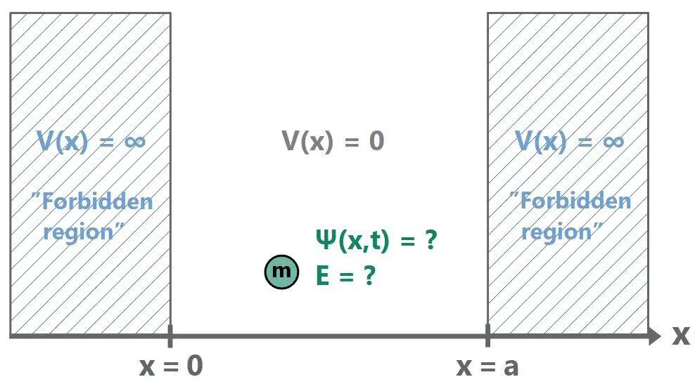
Okay, let’s get started. We’ll consider a particle of mass m confined to an infinite potential well of width a, with potential V(x) = 0 inside the well (0<x<a) and V(x) = ∞ outside. In practice, an “infinite” potential just means the particle can physically never be found outside the well.
Inside the well, the potential is zero, so the time-independent Schrödinger equation takes the form:
-\frac{\hbar^2}{2m}\frac{d^2\psi(x)}{dx^2}+V(x)\psi(x)=E\psi(x)\ \Rightarrow\ \frac{d^2\psi(x)}{dx^2}=-k^2\psi(x)Here, we’ve defined k=\sqrt{2mE}/\hbar – also called the wavenumber. The energies are therefore E=\hbar^2k^2/2m.
This is a very standard ordinary differential equation (ODE), which has a general solution of the form:
\psi(x)=A\sin(kx)+B\cos(kx)So, we’ve solved the time-independent Schrödinger equation for ψ(x). The next step is to apply boundary conditions (which is a part of solving the TISE) to find the energies and the coefficients A and B.
Boundary Conditions, Quantization & Normalization
Due to the potential being infinite outside the well, the wavefunction must go to zero at the walls. This imposes the boundary conditions:
\psi(0)=0\\\psi(a)=0Imposing these condition on the solution ψ(x) from above, we have:
- At x = 0: \psi(0)=A\sin(0)+B\cos(0)=B=0. Thus, \psi(x)=A\sin(kx).
- At x = a: \psi(a)=A\sin(ka)=0, and assuming A ≠ 0, we require ka=n\pi,n=1,2,3,... or k_n=n\pi/a.
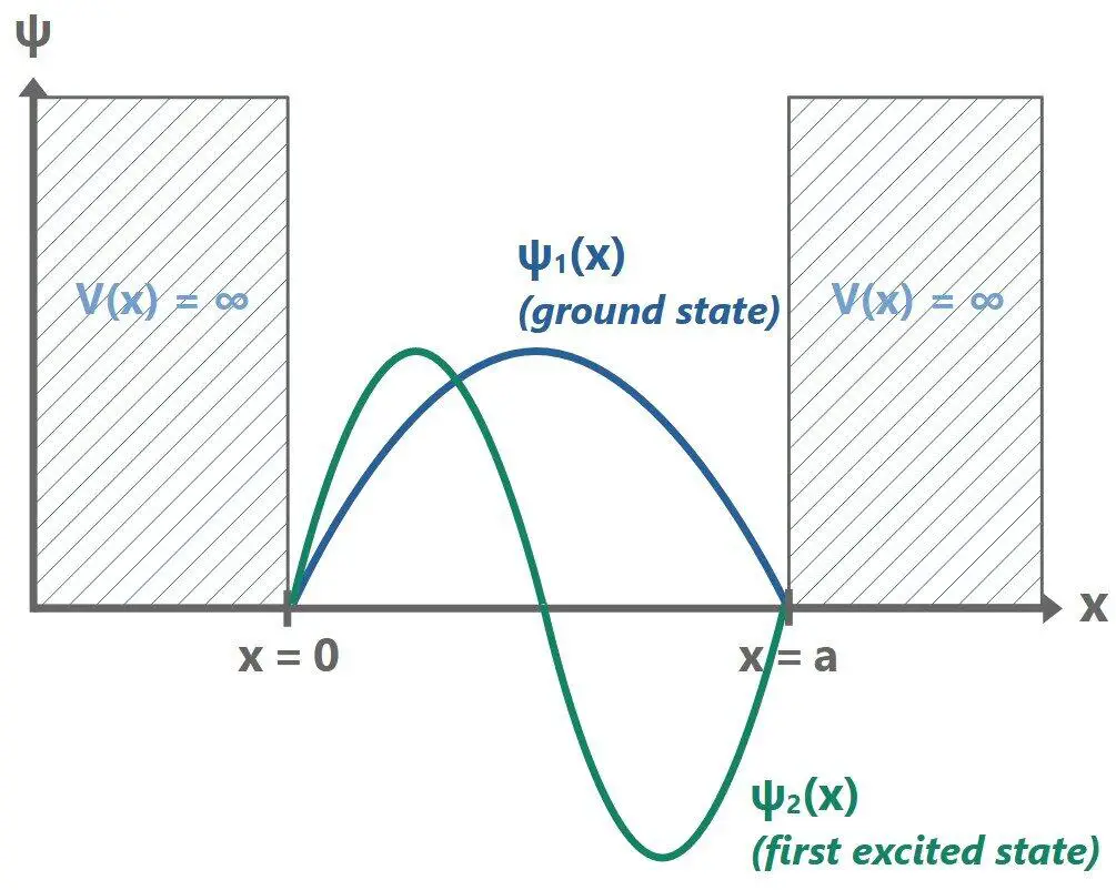
With these, we find the energies as E_n=\frac{\hbar^2k_n^2}{2m}=\frac{\pi^2\hbar^2}{2ma^2}n^2 and the spatial wavefunctions as \psi_n(x)=A\sin(\frac{n\pi x}{a}).
Let’s pause here for a moment and think about what we’ve found. We’ve found the solution to the TISE (spatial wavefunctions and energies), which by completeness, should give us the general solution of the TDSE.
Physically, the boundary conditions fix the coefficient B as well as the energies. We see that
the energy cannot be any arbitrary number (like the way we are used to in classical physics), rather, its values are “spaced out” discretely based on the number n: the energies of the particle are quantized.
To fix the coefficient A, we still have an additional condition; the wavefunction must be normalized. This gives:
\int_0^\infty|\psi_n(x)|^2dx=\int_0^a|A|^2\sin^2(\frac{n\pi x}{a})dx=|A|^2\frac{a}{2}=1\ \Rightarrow\ A=\sqrt{\frac{2}{a}}Finally, we have:
\psi_n(x)=\sqrt{\frac{2}{a}}\sin(\frac{n\pi x}{a})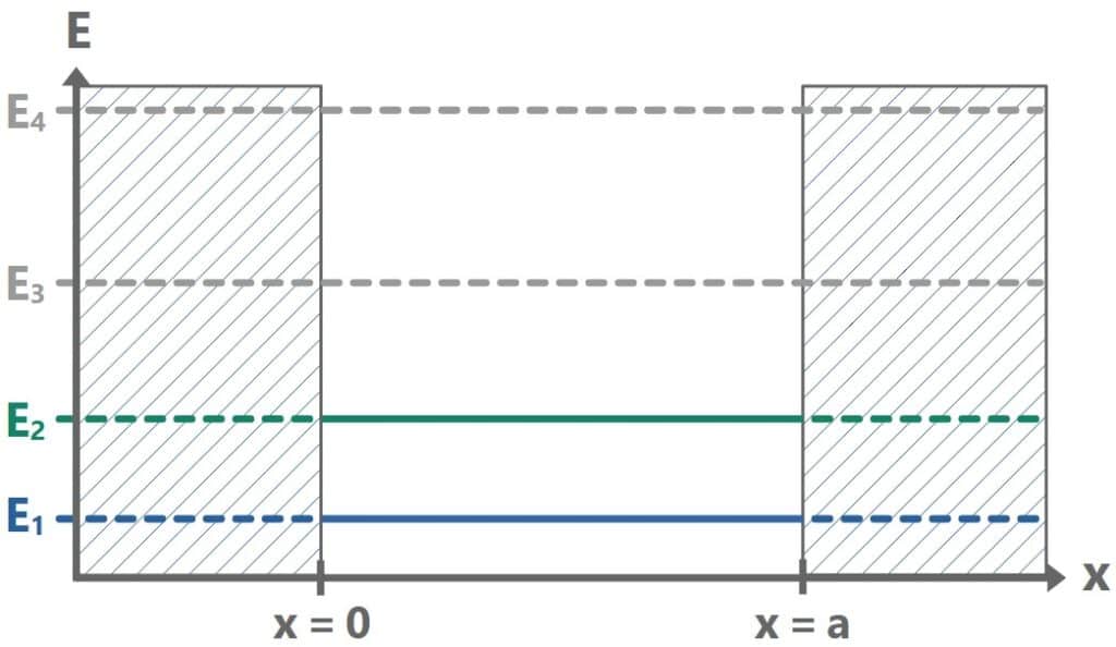
The Full Time-Dependent Solution
Now that we’ve solved the TISE for the spatial part of our wavefunction, adding the time-dependence is simple: we just tag on the temporal wavefunction we’ve already solved, T(t) = e-iEt/ℏ.
The important part is that both the spatial and temporal solutions share the same energy E. This means the temporal function will also be quantized and have an index n denoting the possible energy level. With that, we have the full stationary state solutions \Psi_n(x,t)=\psi_n(x)T_n(t):
\Psi_n(x,t)=\sqrt{\frac{2}{a}}\sin(\frac{n\pi x}{a})e^{-\frac{iE_nt}{\hbar}}
Okay, we’ve found the full stationary state solutions! Now, for a given n, the above Ψn(x,t) represents just one (separable) solution. The most general solution of the full time-dependent Schrödinger equation would be a linear combination of all such solutions:
\Psi(x,t)=\sum_{n)=1}^\infty c_n\Psi_n(x,t)=\sum_{n)=1}^\infty c_n\sqrt{\frac{2}{a}}\sin(\frac{n\pi x}{a})e^{-\frac{iE_nt}{\hbar}}
Mathematically, the coefficients cn are determined by the initial wavefunction Ψ(x,0) as c_n=\int_0^a\psi^*_n(x)\Psi(x,0)dx. And, since Ψ is supposed to be normalized, we have the additional constraint \sum_n|c_n|^2=1.
Below, you’ll find an interactive plot to play around with the general wavefunction shown above. You can specify the coefficients cn and see how the probability |Ψ(x,t)|2 evolves in both space and time (the graph shows the probability, not the complex wavefunction itself). Clicking the Play-button next to the time slider shows an animation of how the probability evolves in time.
Try yourself: set the list of coefficients to c = [1,0,0,0,0,0,0,0] and c = [0,1,0,0,0,0,0,0], which correspond to the stationary states ψ1(x) and ψ2(x) (i.e. the ground state and the first excited state). If you now press Play, you’ll see that the probability doesn’t change with time, which illustrates the idea of a stationary state. How would the stationary state ψ3(x) look like?
Key Takeaways From The Example
- The problem began by defining a potential and setting up the time-independent Schrödinger equation (TISE). In the region inside the well, we had:
- The boundary conditions ψ(0) = ψ(a) = 0 and normalization condition provide us a unique solution to the TISE, as well as quantized energy levels for the system: E_n=n^2\pi^2\hbar^2/2ma^2.
- The full stationary state solutions for a given energy level n – which are solutions to the TDSE – then take the form:
- The most general solution to the problem is obtained as a superposition of all stationary states, by completeness:
Abir Ghosh
I’m a PhD student at the Indian Institute of Science. My research focuses on the early universe and decoding holography – not the sci-fi kind with glowing projections, but the kind that suggests that all our stories are written on the edge of spacetime. When not wrestling with quantum fields or pretending the universe makes sense, you’ll find me trekking the Himalayas, playing the flute, singing (sometimes on key), or consuming cinema and anime.
This article has been co-authored by Abir Ghosh.