The subject of calculus is often seen as somewhat intimidating or difficult, but it really isn’t once you get the hang of it and the big thing about this is to understand why we use calculus in the first place.
Calculus, or mainly differential calculus (integral calculus is a whole different thing), is all about describing how things change.
Now, even though differential calculus itself is just math, I want to introduce it here in terms of physics to hopefully give you motivation as to why differential calculus is needed anyway.
In physics and especially mechanics, we’re often interested in how physical objects and systems move and behave under change.
Calculus is the mathematical language to describe all of this. For example, in physics we may want to describe how the position of an object changes with time and for this, we need calculus.
Now, at the center of differential calculus is the concept of a derivative, which is what we’ll talk about next.
Introduction To Derivatives
To put it simply, a derivative is a mathematical tool used to describe how something changes in relation to something else. In the simplest cases, derivatives describe how a function of some variable changes as you change this particular variable.
In physics, we may often want to describe how a certain quantity changes with time and for this, we need to take the derivative of this quantity with respect to time. In other words, this time derivative describes how the particular quantity we’re interested in changes as time changes (moves forwards).
A great example of this is the velocity of an object, which is defined as the time derivative of position:
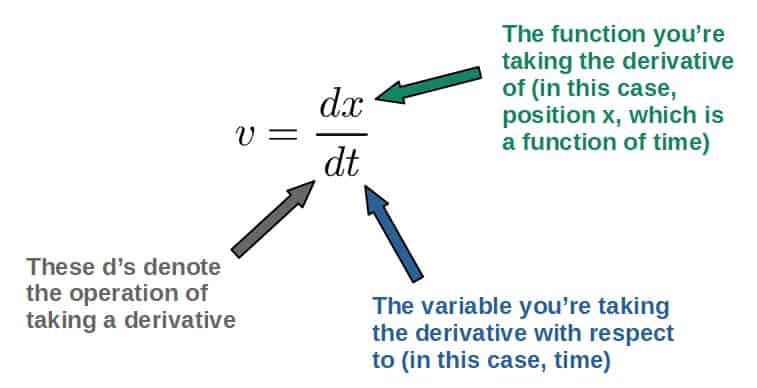
Now, velocity is the time derivative of position as it describes how position changes with time (which is what a derivative does). But still, why a derivative? Why not just “distance divided by time” like we’re used to from elementary physics classes:
The problem with this is that it only gives an average velocity. Sure, you could move a distance of 50 meters in 10 seconds, in which case the velocity would be 5 m/s, but this would only give the average over the period of 10 seconds. It would not account for the fact that you may move the first 5 seconds with a velocity of 3 m/s and the other 5 seconds with a velocity of 7 m/s. The average is still 5 m/s.
So, instead of looking at averages over “long” periods of time, we’re going to look at really really small changes over really small periods of time, essentially giving us the velocity at a single point in time.
Think of it this way; the smaller the change we’re looking at at any given time, the more accurately it’s actually going to describe the situation (formally, we would take the “limit” as these changes get “infinitely” close to zero, which in principle, would give a perfectly accurate result).
This is exactly what a derivative does. It’s a measure of how a quantity changes with respect to an extremely small change in another quantity. This is, in fact, what the d’s in the derivative signify:
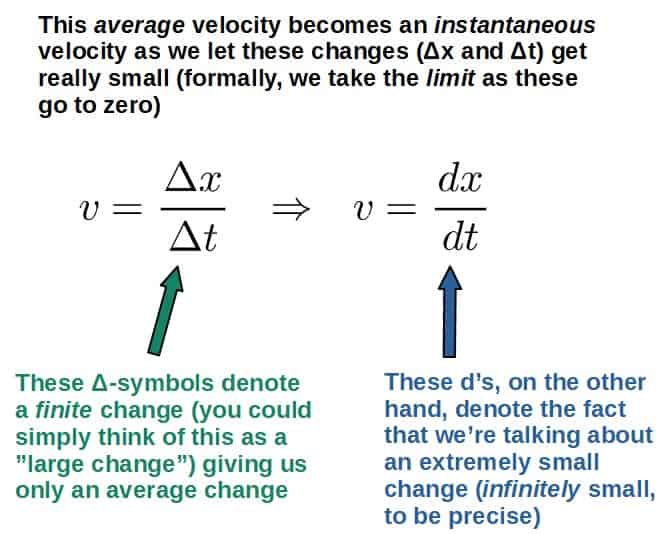
In the case of velocity, this allows us to describe the velocity of any object over shorter and shorter time periods and if the time period is short enough, we’re pretty much talking about velocity at a single instant of time (instantaneous velocity).
In physics, we’re usually not interested in averages over a period of time but rather how a quantity changes from one instant of time to the next (if we know all of these small changes, we can also predict how the quantity behaves over “longer” periods of time, which is what integrals do, but more on that in the next lesson).
This is why pretty much everything in physics will be described by derivatives. If you’re not quite comfortable with this concept yet, don’t worry.
For now, you could simply think of derivatives as mathematical tools to describe how things change, because this is how we’ll usually treat them. They are simply tools to help us form equations (these are called differential equations), which we then need to solve to actually describe the physics involved.
Derivatives In Physics: What You Can Expect
Let’s continue our discussion of derivative in physics. We’ll later talk more about the math associated with taking derivatives of functions
In physics, derivatives will appear all over the place once you get beyond the basic elementary level concepts.
In reality, nature and the laws of physics are described by what are called differential equations. These are equations involving derivatives of different quantities, which we then have to solve to describe how these quantities behave.
As an example, Newton’s second law (F=ma), which you may already be familiar with in some form or another, is really a differential equation that involves the second derivative of position with respect to time (this is how the acceleration a is defined in the language of differential calculus):
We’ll be looking at how to solve such a differential equation (by using integrals) briefly in the next lesson.
Anyway, for now the key point is that physics is described by differential calculus. Down below I’ve collected some of the most common types of derivatives you’ll encounter (both in this course and in other areas of physics).
Time Derivatives
One of the most common and most important forms of derivatives you’ll encounter in physics are time derivatives. In fact, we already discussed these earlier with the example of velocity as the time derivative of position:
In reality, this is actually only the x-component of the velocity since it is the time derivative of the x-position of some object. We could just as well have dy/dt, which would be the y-component of velocity. Moreover, velocity is also a vector quantity and this does not account for that.
The more general formula for velocity would be as follows:
More generally, we could take the time derivative of any quantity, which would describe the time rate of change of that quantity.
Another example of a time derivative is force, which is actually defined as the time derivative of the momentum vector:
And yet another example is the time derivative of energy, which actually gives the dot product of force with velocity:
The main point with all of these is that time derivatives always describe the rate of change of some quantity with respect to time, which is what we’ll want to know in physics.
Second & Higher Order Derivatives
We can also take the derivative of a derivative. Now, what do I mean by this?
An example would be the time derivative of velocity (dv/dt), which is acceleration (denoted by the vector a). But remember that velocity in itself is the time derivative of position. So, we’re basically taking the time derivative of a time derivative:
The derivative of a derivative is called the second derivative. In this case, it’s the second derivative of the position vector r with respect to time and we denote it as follows:
In principle, we could also take the time derivative of acceleration, which would give the third time derivative of position. Such a thing actually exists and it’s called jerk, but it does not have all that many practical uses.
In fact, we could theoretically have any order of a time derivative we wish (the order of a derivative basically means how many times a derivative is taken; for example, acceleration is a second order time derivative), but the practical applications of third or higher order derivatives are not very many, which is why you’ll almost never encounter them in physics and not too often in mathematics either.
Positional Derivatives
So far, I’ve pretty much only talked about time derivatives. However, we may also have a derivative of something with respect to any other variable/quantity.
Another quite common thing you’ll see is the derivative of something with respect to position. For example, a conservative force can be written as the derivative of a potential with respect to position, meaning that the force is actually a measure of how the potential changes with position:
Now, the problem with something like this is that in three dimensions, position is a vector quantity (the position vector r). However, taking a derivative with respect to a vector is quite a weird idea and it requires a slightly different approach.
The approach to this is know as the gradient, which allows us to take derivatives with respect to position even in three dimensions. We’ll discuss the gradient in great detail in the upcoming lessons on vector calculus.
Now, in vector calculus, we’ll generally be interested in taking derivatives of vectors with respect to coordinates (such as x, y and z).
You could think of these as “derivatives with respect to position”, but mathematically it is what it is; a derivative with respect to a coordinate, which may or may not have any physical meaning.
Rules For Taking Derivatives
Now that we’ve talked about the basic idea of derivatives and what they mean from the physics perspective, it’s time to answer the question; how do we actually take derivatives?
For this, I’m going to present you with some rules and some examples of how to use them. If you want, you can find the proofs of these quite easily online.
Also, for these examples, we’ll be looking at single-variable functions only (in later lessons, we’ll look at multivariable functions and how to deal with these).
Basic Derivative Rules
Let’s assume that we have two functions f(t) and g(t), which are functions of the variable t (could be time, for example). Then, the derivative of the sum of these two is simply the sum of the derivatives:
In other words, derivatives can be “distributed” on a sum of multiple terms like this.
Let’s say we have a function of the form:
The derivative of this would then be simply:
Here we can distribute this derivative to get:
In a few sections, I’ll explain how to take the derivatives of each of these terms, but the point here was that if we have a sum of any number of stuff, we can distribute the derivative operator individually to each of the terms.
Another important property is that the derivative of a constant is always zero (which is because constants don’t change by definition and if something does not change, it’s derivative is zero):
Based on this, if we have a function with any constant coefficient, this coefficient can be moved “outside” the derivative since it doesn’t affect taking the derivative in any way:
Power Rule
Probably the most simple rule for actually taking derivatives you’ll encounter is the power rule, which applies to any function that has a constant exponent. For example, all polynomials are of this form, but more generally, also square roots and negative exponents satisfy this rule.
The power rule states that the derivative of any function of the form tn (where n is any constant number, fractional and negative also work) can be calculated as:
In other words, all you do with this when taking a derivative is bring down the original exponent to be a coefficient and then reduce the exponent by one.
As an example, consider the following function:
Now let’s take the derivative of this function:
As we learned earlier, if we have a sum of terms, we can distribute the derivative to each term individually:
We can also pull out any of these constant coefficients (from the first and second terms):
Now I’ll write these terms in the following way by explicitly writing their exponents (t=t1, √t=t1/2 and 1/t2=t-2). This makes it easier to take the derivatives:
Then we just apply the power rule. From the first term, we bring down the exponent of 1 and reduce the old exponent by one (giving us zero and anything to the power of zero is just 1):
From the second term, we bring down the 1/2 and reduce the exponent by 1, giving us -1/2 (which, of course, is the same as 1/√t):
From the last term, we bring down the -2 and reduce the exponent again by 1, giving us -3 (which is just 1/t3. Also, don’t forget the minus sign we originally had in front of this last term in the function):
We now have all of the terms, so the final derivative of this function is then:
In this example, I purposefully wanted to be very explicit in these calculations, but when we move on, I’ll be assuming that you know how to use this rule when needed. Don’t worry though, you’ll be able to get lots of practice from doing the practice problems from the workbook after this lesson.
Product Rule
Taking the derivative of a sum of terms is quite simple, we just take the derivative of each term individually. But what about the derivative of a product? It’s not quite as simple, but luckily still not very involved.
The derivative of a product requires us to use the product rule (a very creative name, right?), which states that the derivative of the product of any two functions, say f(t) and g(t), is:
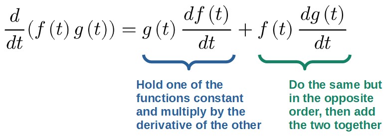
You could think of the product rule as basically saying “how does this product of two functions change as a whole with respect to the variable t”? The first term would then measure the change in f while g is constant and the second term would measure the change in g while f is constant. The total change is then the sum of these two.
Anyway, the product rule is actually quite simple to use. Down below you’ll find an example of using it.
Consider taking the derivative of the following thing:
In principle, you could just multiply out these parentheses and then only use the power rule, but it may be easier to just use the product rule and then the power rule. So, we clearly have the product of two functions here. Let’s define the first as f(t) and the second as g(t):
We then apply the product rule:
Let’s calculate these derivatives term by term. First, we have df(t)/dt:
Now, we just use the power rule for these terms to get (also note that the derivative of a constant, in this case 1, is zero so the last term goes away completely):
Okay, now let’s do dg(t)/dt:
Then, apply the power rule again to each of these terms to get:
We now have everything we need. Just insert these into the formula for the product rule and we get:
If you wish to, you can multiply out these terms and simplify, but it’s fine to leave this as it is right now.
Chain Rule (For Single-Variable Functions)
The last basic rule for derivatives we’ll need is the chain rule, which has to do with composite functions. Basically what this means is that we have a “function inside another function”. An example of this could be:
Here, we have a function f(t)=3t+1 inside the function g(t)=t2. Why? Well, you can check by plugging f(t) into g(t) and you’d get h(t). Now, these composite functions may sometimes be a little difficult to recognize, but you’ll get better at it by practicing.
Anyway, the way to take derivatives of these composite functions is by the chain rule, which states the following:
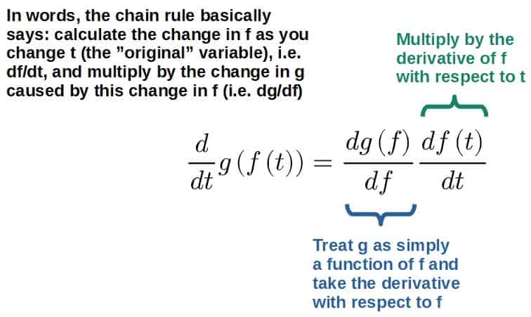
Now, this may seem quite complicated at first, but honestly, it’s quite easy in practice. A nice way to remember all of this, which I use also sometimes is to think of these derivatives as simple fractions:
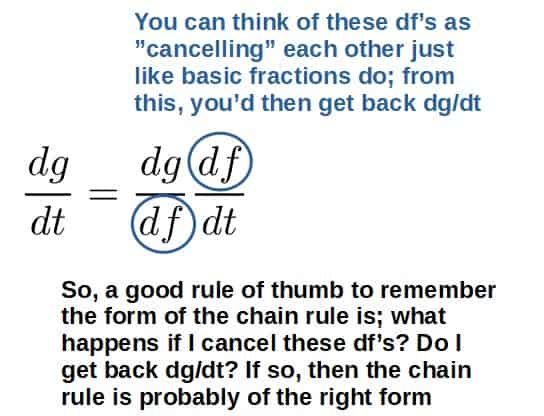
Now, how do you actually use the chain rule in practice? You’ll find an example of this down below and some practice problems in the workbook.
Consider the function h(t):
Here, we can see that this can be viewed as a composite function. Namely, the function f(t)=2t2+t inside the function g(t)=√t. Based on this, we could write h as:
In other words, we now have g as a function of f i.e. g=g(f), which is what we use for the chain rule. The derivative of h would then be:
Now, let’s look at each of these terms. First, we need g(f), which is just:
Now, take the derivative of this with respect to f (simply using the power rule):
Then, for the chain rule, we also need df(t)/dt (f(t) being simply 2t2+t):
We can then plug these into the chain rule formula:
Now, one last thing, which is to plug in the function f:
It may also be enlightening to look at the result in full. So, we took the derivative of √(2t2+t) to get:
Basically, the process we did was:
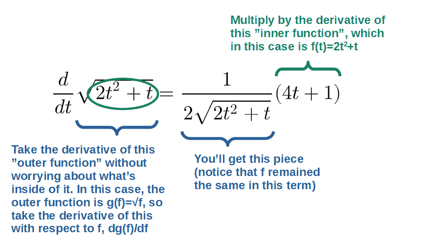
Something to note is that if we have functions of multiple variables, the chain rule becomes a little more complicated (but still quite straightforward once you get the hang of it). We’ll look at this in the lessons on multivariable calculus.
Useful Derivative Formulas
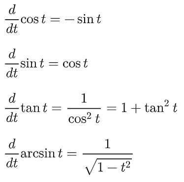
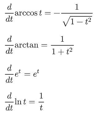
There are also a handful of other useful derivative rules, namely for the derivatives of a few specific functions. These are the following:
Lesson Summary & What To Do Next
Here’s a quick summary of this lesson:
- Differential calculus is the mathematical language to describe change. This is why calculus is used all throughout physics as it allows us to describe how a quantity changes with respect to another quantity (such as time).
- The central concept of differential calculus is the derivative. A derivative of some function f(t), denoted as df(t)/dt, describes how f(t) changes due to a small change in the variable t.
- Derivatives can generally be with respect to any variable, but the most common ones in physics are time derivatives and positional derivatives.
- In vector calculus, we will often take derivatives of vectors with respect to different coordinates.
- It’s also possible to have derivatives of derivatives, which are called second derivatives. An example of this is acceleration (which is the second time derivative of position).
- The basic rules for derivatives are the addition rule, the power rule, the product rule and the chain rule. There are also specific rules for a few specific functions, such as for the various trigonometric functions.