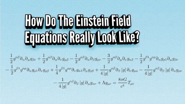
The Friedmann Equations Explained: A Complete Guide
Fewer than 10 years after Einstein’s derivation of his famous field equations, there were already several exact solutions known, including the Friedmann–Lemaître–Robertson–Walker (FLRW) solution, describing an expanding universe.
In 1922, Alexander Friedmann derived two equations beginning from the Einstein field equations and the FLRW solution that now go by the name of the Friedmann equations.
The Friedmann equations are a set of dynamical equations describing the expansion of the universe based on its matter content. The Friedmann equations provide a model for describing many of the observational features of the universe and are widely used throughout modern cosmology.
Naturally, this article finds its place in the playground of general relativity, which at first glance may seem intimidating. However, everything discussed throughout this articles comes from very few, simple assumptions and observations.
This article will be an in-depth view at these assumptions and their implications, providing you with a foundation in Friedmann models of cosmology, the Friedmann equations as well as their applications.
Whilst I will try to explain everything as simply as possible, a previous encounter with the language and tools of general relativity would be beneficial.
For this, you can read my introductory article General Relativity For Dummies that covers everything you need to know to understand this article.
Note that you can get this article and my other general relativity articles in downloadable PDF form here.
With all this being said, let’s begin with an intuitive overview of the Friedmann equations and Friedmann cosmology. We will then dive deeper into the details later.
Table of Contents
Introduction to Friedmann Cosmology
Now that the James Webb Space Telescope (JWST) is up and running, I want you to imagine that for a day you have control over the telescope. You might be curious to find the first Messier object, the Crab Nebula – the remains of the explosive death of a star, a supernova witnessed on Earth around a thousand years ago.
Maybe your astronomical wishes are humbler and you want to observe Jupiter’s Great Red Spot, a great and ancient storm ravaging across the gas giant’s face.
The universe contains many wonders to explore and observe if you just look close enough. But what happens if you do the opposite and you want to zoom out and take a less specific glimpse at the universe?
You would most likely find that, whichever direction you point your telescope, the universe would look pretty much the same. And here we find the first of our assumptions – the property of isotropy.
- Isotropy: On large scales, the universe looks the same in all directions. There is no preferred direction.
Why might we assume this? Well, this relates to one of the observations we can make: the universe is expanding.
The direction of the arrow of time itself is a big area of study in theoretical physics but for all intents and purposes we can say that time is flowing forward, it increases. And as time increases, we see the universe expanding.
What happens if we wind back the clock? The universe starts shrinking.
If we follow this line of thought, we arrive at the universe starting from a singular point – we have stumbled across the Big Bang!
If the universe did start from a Big Bang like this and then expanded outwards, there would be no reason for there to be a preferred direction of expansion (I discuss this more in my article Did The Big Bang Happen Everywhere At Once?).
Quantum fluctuations in the early universe, due to the unpredictable and jiggling nature of fundamental particles, would have effects observable on smaller scales (the size of galaxies and smaller) but on the whole, everything should look rather the same.
Now, we happen to have built the JWST on Earth. Luckily, today you are in control of the telescope and you are able to pick it up, place it down somewhere else in the universe, far away from Earth, and then get your broad-view images back.
Again, you look at them and they appear almost exactly the same as those on Earth. This is our second assumption in Friedmann cosmology – homogeneity.
- Homogeneity: On large scales, the universe appears the same in all locations. There is no preferred location.
The two assumptions we have made are called the cosmological principle and this is what Friedmann and others took as their basis to solve Einstein’s field equations.
We can use the cosmological principle to tackle Einstein’s field equations,
G_{\mu\nu}=\frac{8\pi G}{c^4}T_{\mu\nu}I have a whole article dedicated to exploring and deriving the Einstein field equations in detail (as well as my introduction to general relativity), however for our purposes, we just need to know the basics.
On the left-hand side of the above equation is all the information about gravity encoded in the geometric language of general relativity and is called the Einstein tensor, Gµν.
The lower “indices” µ and ν are the Greek letters “mu” and “nu”. They appear here since the Einstein tensor isn’t just a single number or a function but instead can be imagined as a matrix (more accurately, a tensor), where each μ and ν run from 0 to 3, meaning we should view it as a 4×4 matrix.
The right-hand side tells us about the matter content of the universe. Tµν is called the energy-momentum tensor. This has different forms depending on the matter we want to put in the universe.
The energy-momentum tensor is then multiplied by fundamental constants of nature respectively related to geometry, gravity, and relativity: pi, Newton’s gravitational constant G, and the speed of light c.
This equation is the main result of Einstein’s theory of general relativity – if we can solve the Einstein field equations, we can describe how spacetime and the matter in it behave.
The intuition behind the Einstein field equations is best summarized in the following quote by John Archibald Wheeler:
“Spacetime tells matter how to move, matter tells spacetime how to bend.”
Now, getting back to the Friedmann equations, they essentially come from solving the above Einstein field equations.
I won’t exactly derive the Friedmann equations here but I’ll point out some observations and key points that go into deriving them. We will also look at some of the mathematics related to this later on.
We went to the trouble of figuring out the cosmological principle so we will start there.
First, the universe is isotropic and looks the same in all directions – as such this translates to the universe being spherically symmetric (mathematically speaking), which drastically simplifies the left-hand side of the Einstein field equations.
Second, the matter content of the universe on large scales is modeled as a perfect fluid. This “perfect fluid assumption” is incredibly important in the case of the Friedmann equations.
This is because a universe modeled as a perfect fluid implies that all matter (again, on large scales) is distributed uniformly – the same everywhere. This is nothing other than homogeneity from earlier!
A perfect fluid also has a convenient and simple energy-momentum tensor (more on this later).
After employing the cosmological principle and a lot of math, we are rewarded with two things:
- The metric, describing the curvature and behavior of spacetime
- The Friedmann equations, describing the behavior of matter and expansion of the universe.
I explore the metric, called the Friedmann-Robertson-Walker (FRW) metric more in the article Did The Big Bang Happen Everywhere At Once?, but I’ll briefly recap the key points here.
A metric is a mathematical object that gives a measure of spacetime distances, which essentially generalizes Pythagoras’ theorem. However, the metric also includes the curvature of spacetime as well as the fact that time and space act a bit differently.
Now in all its glory, here is the FRW metric (or more accurately, the line element of the metric):
ds^2=g_{\mu\nu}dx^{\mu}dx^{\nu}=-c^2dt^2+a^2\left(t\right)d\mathbf{x}_{space}^2The left-hand side (ds2) is short for an infinitesimally small distance squared and the right-hand side describes how the different coordinates in spacetime change.
The middle is just a more general, shorthand way of writing the right-hand side and we can refer to just gμν as the metric as it contains all the same information as ds2.
We’ll discuss this line element in a bit more detail later.
Most importantly, a(t) here is called the scale factor and it determines how large-scale distances in space change with time. The scale factor is the most important part of the Friedmann equations and it will appear again and again throughout this article!
The most important property about a(t) is that it only depends on time (it affects all of space in the same way as time passes) and that as you rewind back in time, a(t) eventually goes to zero – the Big Bang singularity!
The scale factor is also explained in more detail later.
Quick tip: If learning more about metric tensors and generally about the math behind general relativity is of interest to you, I would highly recommend checking out my Mathematics of General Relativity: A Complete Course (link to the course page).
This course aims to give you all the mathematical tools you need to understand general relativity – and any of its applications. Inside the course, you’ll learn topics like tensor calculus in an intuitive, beginner-friendly and highly practical way that can be directly applied to understand general relativity.
An Intuitive Explanation of The Friedmann Equations
After completing the Herculean task of creating a cosmological spacetime model through the cosmological principle and the FRW metric, let’s see what we can learn from it and how the Friedmann equations come about from it!
Without further ado, here are the Friedmann equations:
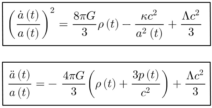
Let’s begin breaking these down! Below, you’ll find an explanation for each term appearing here in the above equations.
However, on a bigger note, the Friedmann equations essentially describe how the scale factor, a(t), changes with time based on the various matter and energy contents we want to put in our spacetime.
The Friedmann equations are two differential equations that can be solved to find the scale factor associated with various models of matter (more on these later).
These solutions, the scale factors a(t), then describe how different types of spacetimes or universes behave based on their matter, radiation and energy content. We will explore some of these solutions later on.
Constants of Nature
Constants of nature appear in almost every equation in physics and they give us small hints about what the equation might be physically representing.
In the Friedmann equations, we have Newton’s constant G, pi, and the speed of light c.
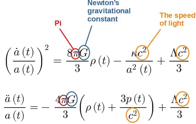
Newton’s constant being present tells us that these equations are likely to involve gravity.
Well, we are describing a spacetime with things in it and thanks to Wheeler’s intuitive explanation of spacetime and matter interacting, combined with Einstein’s interpretation that gravity is geometric, we expect gravity to make an appearance.
Whenever geometry and any kind of spherical shapes are involved, pi is never far behind.
The formula for a circle’s circumference, namely circumference = π x diameter, tells us (after rearranging) that the constant π is defined as the ratio of a circle’s circumference to its diameter.
Now think back.
The cosmological principle tells us that the universe is spherically symmetric – pi will naturally turn up!
Finally, there’s the speed of light, the speed limit of the universe.
Special relativity is based upon the idea that all inertial observers will agree on the speed of light when they measure it. This is explained more in my introduction to special relativity.
This is one of the cornerstones of relativity, so the appearance of the speed of light in the Friedmann equations tells us that these equations likely have something to do with relativity (as expected, of course)!
Altogether, these constants inform us that our equations are about gravity, relativity, and geometry – they could do nothing other than describe a spacetime according to Einstein’s general relativity!
The Scale Factor
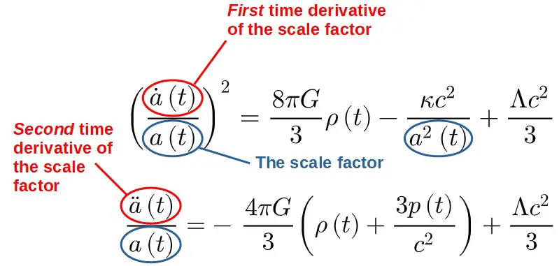
In the Friedmann equations, we see the scale factor a(t) as well as the scale factor with dots above it.
The dot or double-dot above a(t) represents one or two time derivatives – they are measures of how the scale factor changes with time.
In the work of Isaac Newton, he stated his famous equation F=ma. The “a” in this case is the acceleration (not to be confused with the scale factor), it is the second derivative of the position function x(t).
When we have two time derivatives, we can then associate them with accelerations.
As such, the second equation is often referred to as the acceleration Friedmann equation.
It is also worth noting that the first one alone is sometimes referred to as the Friedmann equation.
Now, you may still wonder what the scale factor itself actually is. Below, you’ll find an intuitive explanation that hopefully clears this up.
Earlier, we discussed how the cosmological principle allows us to solve the Einstein field equations and obtain the FRW metric, which describes a spacetime model for the universe and its expansion.
A nice mental image of a universe model according to the cosmological principle is to imagine an infinite grid of dots. The layout of the dots should be the same everywhere and from all directions (the dots have the same distance between each one) – this represents the cosmological principle.
These dots simply represent “points” within space (not spacetime). Effectively, this infinite grid of dots represents the universe – these dots could be galaxies on a large scale, for example.
Now choose a pair of dots and think of a line joining them and that the line is described by some number. We can interpret this number as the distance between points in space (distance between two galaxies, for example).

How is this useful? Well, the scale factor is used to model how the numbers representing the distance between each point in the universe changes with time.
Now, in general relativity, the solutions to the Einstein field equations are always metrics or line elements, describing distances in spacetime.
Line elements are essentially generalizations of Pythagoras’ theorem that describes distances in a typical Euclidean space. Let’s briefly recall Pythagoras’ theorem:
a^2+b^2=c^2These relate the three sides of a triangle, where c is the length of the hypotenuse – however, this formula does more than that.
If we imagine a as the difference in the x-coordinates of two points and b as the difference in the y-coordinates of these points, then this is secretly telling us that the shortest distance between those two points is the straight line, the hypotenuse c, connecting them.
We can generalize this to points in 3D where we would have a2+b2+c2=d2. Now the shortest distance between the two points is d and c is the difference in the z-coordinates of the two points.
If we talk about space, it is convenient to talk about very small (infinitesimal) distances and we would write:
ds^2=dx^2+dy^2+dz^2You can think of dx as something like “a small difference in the x-coordinate”. This is what we call a “line element” – it tells us about the distance between two close-by points.
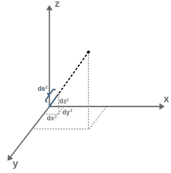
If we were to write a new line element,
ds^2=3^2\left(dx^2+dy^2+dz^2\right)we would triple the distance between the points compared with our original ds2.
This idea of changing distances between points and how the line element encodes them is key in understanding the scale factor.
Now, these line elements describe a space, but not a spacetime like we would want in general relativity – there’s no time component! We add this in like with spatial components but with a subtle change, like this:
ds^2=-c^2dt^2+dx^2+dy^2+dz^2Time has a different sign in front of it! This is because time acts fundamentally differently compared with space – we can’t move freely through time like we can jump up and down or run side to side – this minus sign is the mathematical way to encode this.
Also, recalling that distance = speed*time, we can see that we need the speed of light here as this (c2dt2) gives the correct units of distance.
This particular line element above describes something called Minkowski spacetime and is the simplest solution to the Einstein field equations as it is the immediate generalization of Pythagoras’ theorem to (flat) spacetime.
Minkowski spacetime is used to describe the laws of special relativity, leading to things like time dilation and length contraction. I cover this in more detail in my article Special Relativity For Dummies: An Intuitive Introduction.
Now, the solution we’re interested in is the FRW metric.
This metric is the particular line element we get with the assumptions given earlier (isotropy and homogeneity – the cosmological principle) and it is the most accurate model for our universe at cosmological scales.
The FRW metric as stated earlier can be expressed as a line element of the form:
ds^2=-c^2dt^2+a^2\left(t\right)d\mathbf{x}_{space}^2From what we just covered, we can recognize that the time component looks pretty usual, there’s nothing
different going on compared to the simple Minkowski spacetime we saw earlier.
The spatial components are where it gets interesting. The dx2space here describes distances in space in whatever coordinate system we happen to be using (we won’t necessarily always have the standard Cartesian x,y,z -coordinate system).
In the simplest scenario, namely in Cartesian coordinates, we have dx2space=dx2+dy2+dz2, which we saw previously.
Now, most importantly for us, we can see that the spatial part of the line element is multiplied by the square of the scale factor, a2(t), which is a function of time.
Essentially, the spatial part of the FRW line element represents the infinite grid of dots that changes scale we discussed earlier, but with the grid now in 3D space.
This is because based on what we saw earlier, we know that if we multiply the spacial parts of the line element (dx2+dy2+dz2) by something, this scales the distance between all points in space.
Well, here we see exactly that – the scale factor a(t) in front of the spacial distance changes with time, which means that the scale of the universe will also change with time.
We can find out the exact form of the scale factor by solving the Friedmann equations for any particular matter and energy configuration in the universe – for example, in a matter-dominated flat universe, we would have the time dependence of the scale factor be:
a\left(t\right)\propto t^{\frac{2}{3}}This describes a scale factor that increases with time – a universe where spatial distances get larger and larger as time passes.
We’ll discuss various solutions to the Friedmann equations in more detail later.
Back to the Friedmann equations – there are four pieces of the puzzle left, ρ(t), p(t), κ and Λ.
The Cosmological Constant
The odd triangle-looking thing appearing in the Friedmann equations, Λ, is the cosmological constant – referred to by Einstein himself as his “biggest blunder”, this mysterious term is a way of including dark energy into our model!

The cosmological constant essentially acts like a form of energy with negative pressure in the universe and drives its expansion. We’ll see how all of this comes about later in the article.
The Curvature Term
The constant κ in the Friedmann equations is called the “scalar curvature” and this encapsulates the basic geometric shape of the universe.
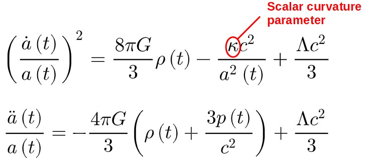
There are three basic types of geometry we can have: Euclidean, hyperbolic, and elliptical.
These can be characterized by different values of the scalar curvature parameter κ:
- Elliptical: κ > 0
- Euclidean: κ = 0
- Hyperbolic: κ < 0
Euclidean geometry is the familiar geometry you may have learned in school where the interior angles in a triangle add up to 180 degrees and so on.
The other two members of the geometry family are a bit more exotic.
For example, the interior angles of a triangle in hyperbolic geometry add up to less than 180 degrees whereas they add up to more than 180 degrees in elliptical geometry!
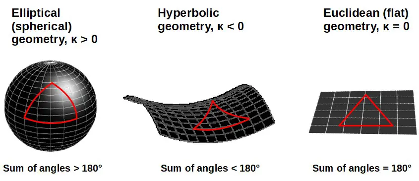
When talking about the universe, we often refer to a universe with elliptical geometry as closed, a universe with hyperbolic geometry as open and a universe with Euclidean geometry as flat.
Now, it’s important to keep in mind that these geometries describe the universe on very large scales only.
For example, when we describe the universe as flat, this is only true at cosmological scales – there can still exist different matter and spacetime curvature configurations on much smaller scales, such as near a single star or black hole.
Pressure and Density Terms
Finally, we have the quantities ρ(t) and p(t) showing up in the Friedmann equations.
Both of these come from the perfect fluid assumption mentioned earlier – p(t) is the pressure of the matter content of the universe and ρ(t) (ρ is the Greek letter “rho”) is the energy density of the universe.
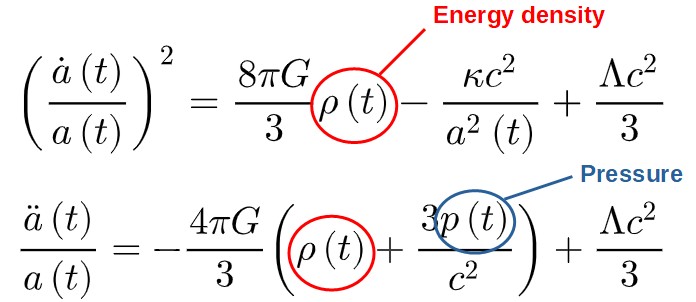
In general, these will both vary with time, which is why they are functions of time here.
We will explore both the energy density and pressure terms in more detail throughout this article and see where exactly they come from and what they represent.
However, it’s worth mentioning that there is a neat way of interpreting the cosmological constant as a contribution to the energy density term with negative pressure.
Let’s make the following two changes to the energy density and pressure of the universe:
\rho\left(t\right)\mapsto\rho\left(t\right)+\frac{\Lambda c^2}{8\pi G}\ p\left(t\right)\mapsto p\left(t\right)-\frac{\Lambda c^4}{8\pi G}The effect of this is “absorbing” the cosmological constant as an additional contribution to the energy density and pressure – we’re effectively just rescaling our variables by a constant amount.
We can see that it takes away from the pressure p(t), hence counting as a negative pressure!
With these variable changes, the new Friedmann equations now read:
\left(\frac{\dot{a}\left(t\right)}{a\left(t\right)}\right)^2=\frac{8\pi G}{3}\rho\left(t\right)-\frac{\kappa c^2}{a^2\left(t\right)} \frac{\ddot{{a}}\left(t\right)}{a\left(t\right)}=-\ \frac{4\pi G}{3}\left(\rho\left(t\right)+\frac{3p\left(t\right)}{c^2}\right)We have one fewer term floating around, which always makes things simpler, and we found a neat interpretation of the cosmological constant along the way.
Where Do The Friedmann Equations Come From?
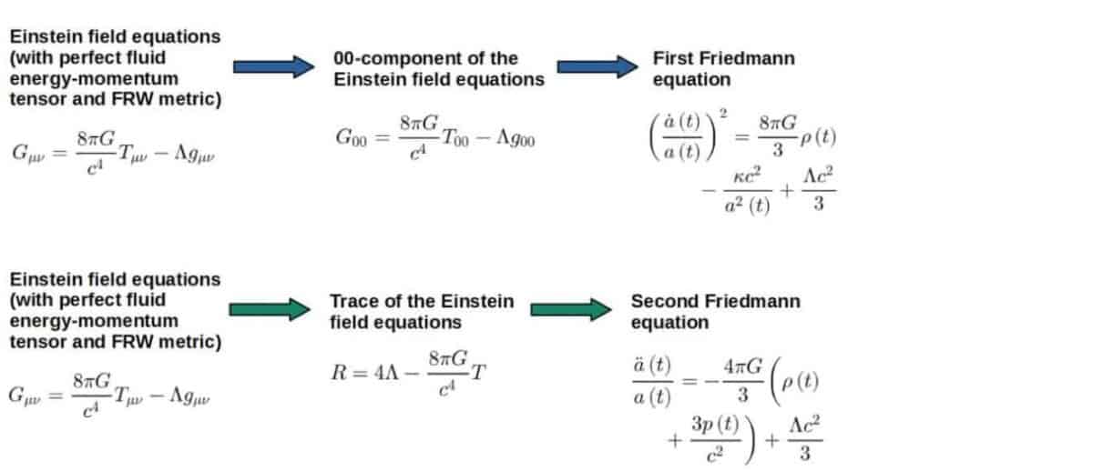
The Friedmann equations themselves originate, as many equations in general relativity, from the Einstein Field Equations (EFEs).
The EFEs describe the evolution of the fabric of spacetime – they tell us how it evolves and changes depending on either the geometry we impose or the matter we put into our spacetime.
Explicitly including the cosmological constant, the EFEs are given by:
G_{\mu\nu}=\frac{8\pi G}{c^4}T_{\mu\nu}-\Lambda g_{\mu\nu}The perfect fluid assumption gives us the following form of the energy-momentum tensor Tμν:
T_{\mu\nu}=\begin{pmatrix}-\rho(t)c^2&0&0&0\\0&p(t)&0&0\\0&0&p(t)&0\\0&0&0&p(t)\end{pmatrix}There are various parameters here but most strikingly the tensor is diagonal – it only has entries along its leading diagonal.
This is a manifestation of the isotropy we mentioned earlier – any off-diagonal elements would describe directional preferences of the pressure and energy density in terms of shear stresses, which would violate our isotropic assumption!
The top-left entry, which we write as T00, describes the energy density of the universe.
This is the interpretation for all energy-momentum tensors, not just our perfect fluid tensor.
In case you’re interested in understanding this in more detail, I cover the physical interpretations of each term in the energy-momentum tensor here.
We’ll talk much more about energy density later but, in effect, it describes all of the matter, dark matter, radiation etc. in our universe – it is the “stuff” part of the universe.
With that in mind, we’d like to describe how the components of the universe – the “stuff” – behave so it makes sense to look at the 00-component of the EFEs,
G_{00}=\frac{8\pi G}{c^4}T_{00}-\Lambda g_{00}If you were to work through and calculate the above equation explicitly (namely, insert the FRW metric g00-component and calculate the Einstein tensor G00-component for the FRW metric), what you get out is exactly the first Friedmann equation!
Now, the second Friedmann equation is a bit more subtle. It actually comes from taking the trace of the EFEs, which gives us a scalar equation instead of a tensor equation.
The Einstein tensor is defined in terms of the curvature of our spacetime. In particular, it involves another curvature scalar called R, the Ricci scalar.
I won’t go into the exact mathematical details here, but after taking the trace of the EFEs, we get the following equation:
R=4\Lambda-\frac{8\pi G}{c^4}THere, R is the Ricci scalar and T is the trace of the energy-momentum tensor (sum of the diagonal matrix elements). Moreover, this is now a scalar equation – we no longer have any tensor indices floating around!
Using this equation, combined with the first Friedmann equation, we can derive the second Friedmann equation.
So, here’s a little summary of where both of the Friedmann equations actually come from in the first place:
The Hubble Constant
There are a couple important parameters that often show up when discussing the Friedmann equations.
Ideally, we’d like to talk both quantitatively and qualitatively about the universe. To do the former, we can do direct calculations but to aid us in the latter, let’s introduce some concepts from cosmology.
Our first concept is the Hubble parameter H(t), defined as:
H\left(t\right)=\frac{\dot{a}\left(t\right)}{a\left(t\right)}This is a convenient renaming of the left-hand side of the first Friedmann equation that will play a part in the rest of this story.
Now, the things that we can measure in the universe are happening at our present time. We’ll call this time t0 (the age of our universe) and all quantities evaluated at this time will be given a subscript 0.
This leads us to the Hubble constant H0, defined as the value of the Hubble parameter at our present time t0:
H_0=H\left(t_0\right)=\frac{\dot{a}\left(t_0\right)}{a\left(t_0\right)}=\frac{\dot{a}_0}{a_0}Note that the Hubble constant is not actually a constant, strictly speaking – its value changes with time since the value of our present time is also changing constantly. However, we can think of the Hubble constant as something that is constant everywhere in space at any particular time.
Hubble’s constant is based on the observation that further away galaxies are travelling away from us at faster and faster speeds. This can be summarized by Hubble’s law,
v=H_0Dwhere v is the velocity of a galaxy’s recession and D is the distance between us and the galaxy.
The next concept is subtler but nevertheless important – it is the density of matter that corresponds to a flat universe today. This is called the critical density ρc.
We are interested in this as current evidence suggests our universe to be flat within a small error margin.
An expression for the critical density can be derived by taking the first Friedmann equation evaluated today at t = t0, inserting the expression for the Hubble constant, setting Λ = 0 and κ = 0 to impose a flat universe, from which we get the critical density:
H_0^2=\frac{8\pi G}{3}\rho_c\ \ \Rightarrow\ \ \rho_c=\frac{3H_0^2}{8\pi G}This expression for the critical density could be evaluated by inserting the current value of the Hubble constant (this gives a critical density value ρc ∼ 10-27 kg/m3), but the exact numerical value isn’t so important here.
The final (I mean it this time) quantity is a dimensionless one, which will later help us rewrite the Friedmann equations to see how different matter populates the universe.
It is the ratio of the density ρ(t) to the critical density ρc and we call it the dimensionless density parameter:
\Omega=\frac{\rho\left(t\right)}{\rho_c}=\frac{8\pi G\rho\left(t\right)}{3H_0^2}With all these parameters at our disposal, we will now move on to discuss various solutions, applications and predictions that the Friedmann equations give us. Let’s go explore the universe!
The Continuity Equation In Friedmann Cosmology
In the Friedmann model of cosmology, we use a perfect fluid with density and pressure (which both appear in the Friedmann equations) to model the matter, radiation and energy content in the universe on cosmic scales, as mentioned previously.
This perfect fluid assumption allows us to encapsulate the cosmological principle.
We’ll talk about how we distinguish these different forms of energy soon, but first, let’s discuss some general properties of the Friedmann equations that applies to all forms of matter.
These properties are encapsulated in something called the continuity equation, which will be hugely important for us later.
Since we’re talking about “a fluid”, it’s useful to also think about how this fluid evolves.
So, imagine a fluid flowing through a pipe. It is completely natural and almost expected that the mass of fluid flowing in is equal to the mass of the fluid flowing out.
In fact, it feels so natural that we might not even think about it – then we had better expect that our model has the same feature.
Well, it turns out that it does and this result is known as the continuity equation. In our perfect fluid, this is the following differential equation:
\frac{\partial\rho\left(t\right)}{\partial t}+\frac{3\dot{a}\left(t\right)}{a\left(t\right)}\left(\rho\left(t\right)+\frac{p\left(t\right)}{c^2}\right)=0The derivation of this is discussed more later.
The continuity equation describes the rate of change of the energy density of the perfect fluid (i.e. of the universe) as the scale factor of the universe changes – it encapsulates the “fluid flowing in = fluid flowing out” property.
In fact, the continuity equation represents the conservation of energy in the Friedmann cosmology model (more on this later).
I will propose that the continuity equation can be rewritten in the following form (this will turn out useful later):
dU=-\frac{p\left(t\right)}{c^2}dVHere, V is a volume in space and U = ρV is an energy density times a volume (i.e. an energy) and the letter “d” in front of variables is effectively a derivative or infinitesimal change like in “dx” earlier.
For those interested, I’ll present the derivation of this below.
The easiest way of showing this equivalence is by starting at the end point and working backwards.
Volumes in space will be affected by the expansion of space itself and so will be proportional to a3(t) (since a(t) represents the spacial distance scale). We can write a volume as V = Aa3(t) for some constant A.
The “d” operates as a derivative and obeys the chain rule and product rule just like the standard derivative operator.
In particular we can follow the following line of equalities,
dV=d\left(Aa^3\left(t\right)\right)=Ad\left(a^3\left(t\right)\right)=3Aa^2\left(t\right)d\left(a\left(t\right)\right)\\=3Aa^2\left(t\right)\frac{da\left(t\right)}{dt}dt=3Aa^2\left(t\right)\dot{a}\left(t\right)dtMany problems in physics can be simplified by multiplying by 1 or adding 0 in different ways.
If we multiply by a(t)/a(t) = 1, we can rewrite this final expression again in terms of V,
3Aa^2\left(t\right)\dot{a}\left(t\right)dt=3\frac{Aa^3\left(t\right)}{a\left(t\right)}\dot{a}\left(t\right)dt=3V\frac{\dot{a}\left(t\right)}{a\left(t\right)}dtThis gives the final expression:
dV=3V\frac{\dot{a}\left(t\right)}{a\left(t\right)}dtLet’s handle the left hand side (with the energy density U = ρV) too by using the product rule:
dU=d\left(\rho\left(t\right)V\right)=Vd\left(\rho\left(t\right)\right)+\rho\left(t\right)dV=V\frac{\partial\rho\left(t\right)}{\partial t}dt+\rho\left(t\right)3V\frac{\dot{a}\left(t\right)}{a\left(t\right)}dtHere, we first use the definition of U, then the product rule and finally insert the expression for dV from above.
Both terms have Vdt in common so we can regroup the terms as:
dU=\left(\frac{\partial\rho\left(t\right)}{\partial t}+3\frac{\dot{a}\left(t\right)}{a\left(t\right)}\rho\left(t\right)\right)VdtNow we’re ready to put everything together!
\left(\frac{\partial\rho\left(t\right)}{\partial t}+3\frac{\dot{a}\left(t\right)}{a\left(t\right)}\rho\left(t\right)\right)Vdt=dU=-\frac{p\left(t\right)}{c^2}dV=-3\frac{\dot{a}\left(t\right)}{a\left(t\right)}\frac{p\left(t\right)}{c^2}VdtOne final rearrangement, taking everything over to the same side gives us
\left(\frac{\partial\rho\left(t\right)}{\partial t}+3\frac{\dot{a}\left(t\right)}{a\left(t\right)}\left(\rho\left(t\right)+\frac{p\left(t\right)}{c^2}\right)\right)Vdt=0The last thing that needs to be pointed out is that Vdt is small but non-zero, so we can satisfy the above equation by demanding that
\frac{\partial\rho\left(t\right)}{\partial t}+\frac{3\dot{a}\left(t\right)}{a\left(t\right)}\left(\rho\left(t\right)+\frac{p\left(t\right)}{c^2}\right)=0And here we have arrived at the original continuity equation! This proves the fact that the differential form of the continuity equation is equivalent to the one above.
Conservation of Energy
What does the continuity equation actually represent? How is it related to energy conservation?
To understand this, we will need to do a little bit of tensor calculus. You can get an introduction to this and general relativity as a whole in the article General Relativity for Dummies: An Intuitive Introduction.
Let’s first think about the fundamental quantity sourcing all of these equations: the energy-momentum tensor Tμν.
So far we have written it with both indices “downstairs” but in the language of general relativity we can raise them “upstairs” using the metric.
If we look at the index-up version of the Einstein field equations, we can see:
G^{\mu\nu}=\frac{8\pi G}{c^4}T^{\mu\nu}-\Lambda g^{\mu\nu}We are at liberty to take the covariant divergence ∇μ of this equation – but why would we?
Well, a non-zero divergence tells us that something is being added or taken from our system, roughly speaking.
Imagine a pond – if you put a geyser in the pond, then there would be a point where water was being added so the total volume of water wouldn’t remain the same.
Similarly, if you add a whirlpool (or plughole), then the water will drain out and also not remain constant!
Mathematically, we describe these by the divergence of a particular quantity.
If we want any chance at getting information related to the continuity equation, we’d like very much to know what happens when we take the divergence of the energy-momentum tensor (and hope that it is zero).
With this picture in mind, here are two facts about the divergence of the Einstein tensor and metric:
- \nabla_{\mu}G^{\mu\nu}=0
- \nabla_{\mu}g^{\mu\nu}=0
Since there are only three terms in the Einstein field equation above and the divergence of two of them is zero, it must also be that the divergence of the energy-momentum tensor is zero:
\nabla_{\mu}T^{\mu\nu}=0Excellent – this feels like we’re on our way to discovering the continuity equation.
There is only one index, ν, not being summed over (remember, when working with tensor indices, repeated indices like μ here are being summed over) which tells us that this is actually four equations, one for each index value of ν:
\nabla_{\mu}T^{\mu0}=0{,}\text{ }\nabla_{\mu}T^{\mu i}=0The i-index here counts i=1,2,3 and labels the spatial components.
The energy-momentum tensor is so named because it describes energy (0) and momentum (i): these two equations describe both the conservation of energy and the conservation of momentum!
Again, you can find more information about the interpretation of the various components of the energy-momentum tensor in the introductory general relativity article linked above.
By Einstein’s famous relation E = mc2, we know that mass and energy can be seen as effectively the same.
The intuitive explanation of the continuity equation involves the same mass entering and leaving an area and since mass and energy are the same, this leads us to look at the conservation of energy equation.
The first equation above with ν = 0 is in fact the continuity equation in disguise!
If you’re interested in seeing this explicitly, have a look at the derivation down below.
The energy-momentum tensor we have is very special to work with as it only has two non-zero types of components (see earlier for the matrix form of the perfect fluid energy-momentum tensor):
- T^{00}=c^2\rho\left(t\right)
- T^{ii}=p\left(t\right)
Let’s consider our conservation equation for the 0-components,
\nabla_{\mu}T^{\mu0}=0This has only one non-zero component, T00, since all terms like Ti0 are zero, hence we can write this using the full definition of the covariant derivative,
0=\nabla_{\mu}T^{\mu0}=\partial_{\mu}T^{\mu0}+\Gamma_{\mu\alpha}^{\mu}T^{\alpha0}+\Gamma_{\mu\alpha}^0T^{\mu\alpha}=\partial_0T^{00}+\Gamma_{\mu0}^{\mu}T^{00}+\Gamma_{\mu\alpha}^0T^{\mu\alpha}In the final term, we can simplify this one step further because unless μ = α, the energy-momentum tensor will be zero, hence
\partial_0T^{00}+\Gamma_{\mu0}^{\mu}T^{00}+\Gamma_{\mu\mu}^0T^{\mu\mu}=0To get out the information we want, we need to know what the Christoffel symbols Γαμν are.
These can be looked up for the FRW universe (I actually have a list of them on this page) and the ones we require can be summarized as:
\Gamma_{i0}^i=\Gamma_{ii}^0=\frac{1}{c}\frac{\dot{a}\left(t\right)}{a\left(t\right)}All other possible combinations of indices in the equation give zero!
This means the conservation of energy equation can be written as
\partial_0T^{00}+\frac{3}{c}\frac{\dot{a}(t)}{a(t)}T^{00}+\frac{1}{c}\frac{\dot{a}(t)}{a(t)}\left(T^{11}+T^{22}+T^{33}\right)=0Plugging everything in, we find:
\frac{1}{c}\frac{\partial\left(c^2\rho\left(t\right)\right)}{\partial t}+\frac{3}{c}\frac{\dot{a}\left(t\right)}{a\left(t\right)}c^2\rho\left(t\right)+\frac{3}{c}\frac{\dot{a}\left(t\right)}{a\left(t\right)}p\left(t\right)=0Finally, by multiplying everything by c and adding brackets, we arrive at the continuity equation I presented before:
\frac{\partial\rho\left(t\right)}{\partial t}+\frac{3\dot{a}\left(t\right)}{a\left(t\right)}\left(\rho\left(t\right)+\frac{p\left(t\right)}{c^2}\right)=0The key point with all of this is that the conservation of energy pops out naturally from the Friedmann equations – it’s built into them.
However, energy conservation is a bit more complicated to interpret in cosmology due to the fact that it depends on how the scale of the universe is changing (this can be seen from the fact that the scale factor appears in the continuity equation).
Still, the continuity equation is the closest we can get to a conservation law for energy and it is extremely useful for predicting how the energy density in the universe evolves.
So, we have the continuity equation that applies to all forms of matter, energy and radiation (modeled as perfect fluids) at our disposal. But of course, not all forms matter, energy and radiation are the same, so how do we distinguish between these?
When talking about matter or radiation, for example, we would intuitively think that density and pressure should be related. But how exactly?
Well, the answer comes from introducing an equation of state.
Equations of State
Equations of state are a crucial part whenever we’re working with the Friedmann equations.
In fact, we cannot really obtain any useful solutions or predictions from the Friedmann equations without an equation of state.
An equation of state simply tells us how different variables are related to each other – in our case this would be energy density and pressure.
In other words, an equation of state relates the density and pressure of any given form of matter or radiation. It describes the “state” of our perfect fluid.
The simplest general equation of state is a linear relationship:

This w here is a parameter that encapsulates information about different types of matter. Also, c is the speed of light once again.
This is what we use to distinguish between different forms of matter and radiation. It is also what allows us to obtain different solutions to the Friedmann equations, as we will see later.
We now have at our disposal both the continuity equation in two different forms as well as our linear equation of state, so we’re ready to analyze what makes up the universe: matter, radiation and dark energy as well as how the Friedmann model of cosmology describes these.
I’ll also present a summary of various solutions of the Friedmann equations for different equations of state later.
Equation of State For Matter
We’ll begin with matter: physically, matter is described as having an energy density much larger than its pressure.
Einstein’s famous equation E=mc2 tells us that mass and energy are equivalent.
However, having a mass isn’t the only form of energy: photons – quanta of light – are massless but still have energy!
Namely, the energy of a photon comes from its momentum, which I explain in my article explaining how photons can have momentum with zero mass.
Knowing these different forms of energy that stuff can have helps us get a grip on why this is a sensible definition of matter.
Both of these forms of energy contribute to the concept of energy density.
However, regular matter in the universe exists without really exerting a noticeable pressure on large, cosmic scales.
Radiation in the form of photons, however, does exert a pressure so it will have a different equation of state (explained soon).
Hence, if the energy density is dominated by the mass density contributions (such as for ordinary matter), the pressure is going to be negligible!
This is the case for planets, moons, even dark matter – it all gets bundled together in what cosmologists call “matter”.
On cosmic scales, regular matter is often modeled as a “dust”, meaning a perfect fluid with no noticeable pressure.
The matter equation of state is therefore given by (so, it has w=0):
p\left(t\right)=0Plugging this in to our second, differential version of the continuity equation gives us:
dU=d\left(\rho\left(t\right)V\right)=0Here, “d” is essentially a derivative or a differential operator, which tells us about how something changes.
A derivative being equal to zero tells us that the thing it is acting on is not changing – it is a constant!
So, the product ρ(t)V here must be a constant here.
However, generally both the energy density ρ(t) and volume V are functions of time, so neither of them is a constant individually – the only way their product can be a constant still is if they both cancel each other out.
This means that ρ(t) and V=Aa3(t) are inversely proportional to one another as this would result in ρ(t)V=constant:
d\left(\rho\left(t\right)V\right)=Ad\left(\rho\left(t\right)a^3\left(t\right)\right)=0With this, we’ve found how the matter contribution to the energy density evolves in time in terms of the scale factor of the universe – it is proportional to a-3(t):
\rho_m\left(t\right)\propto a^{-3}\left(t\right)The interpretation of this is that the energy density of matter gets diluted as the universe expands.
In fact, this result may not be too surprising since in this case, the energy spreads out in much the same way as things on Earth do – imagine filling a square box of side length L with a gas. Let’s say the gas has mass M.
The volume of the box is then L3 and the density of the gas is M/L3 – if we increase the side length, we dilute the gas, with its density scaling as ρ ∝ L-3!
This is exactly what is happening with regular matter on cosmic scales as the universe expands.
Equation of State For Radiation
We can play the same game with radiation. The equation of state for radiation turns out to be (so, w=1/3):
p\left(t\right)=\frac{1}{3}c^2\rho\left(t\right)This equation of state is a result of the properties of the energy-momentum tensor for a general electromagnetic field – namely, the trace of the energy-momentum tensor is always zero for an electromagnetic field.
Therefore, if the radiation we’re discussing here is electromagnetic radiation, this property must also hold for the energy-momentum tensor of our radiation modeled as a perfect fluid.
The trace of the energy-momentum tensor is just the sum of the diagonal elements and this being zero gives:
T_{\mu\nu}=\begin{pmatrix}-\rho(t)c^2&0&0&0\\0&p(t)&0&0\\0&0&p(t)&0\\0&0&0&p(t)\end{pmatrix}\ \ \Rightarrow\ \ -\rho\left(t\right)c^2+3p\left(t\right)=0This, we can of course just rearrange to give us the radiation equation of state presented above.
Now, from this equation of state and the continuity equation, we find that the energy density of radiation (such as a photon gas) still dilutes as the universe expands but differently than regular matter:
\rho_r\left(t\right)\propto a^{-4}\left(t\right)From this, we actually see that the energy density of radiation in the universe decreases faster than that of regular matter (by an additional power of 1/a(t)).
For the full derivation of this result, see below.
If we take our equation of state, p(t)=1/3ρ(t)c2, and plug it into the continuity equation (now the differential equation form), we get the following:
\frac{\partial\rho\left(t\right)}{\partial t}+\frac{3\dot{a}\left(t\right)}{a\left(t\right)}\left(\rho\left(t\right)+\frac{p\left(t\right)}{c^2}\right)=0\\\Rightarrow\ \ \frac{\partial\rho\left(t\right)}{\partial t}+\frac{3\dot{a}\left(t\right)}{a\left(t\right)}\left(\rho\left(t\right)+\frac{\frac{1}{3}c^2\rho\left(t\right)}{c^2}\right)=0\\\Rightarrow\ \ \frac{\partial\rho\left(t\right)}{\partial t}+4\frac{\dot{a}\left(t\right)}{a\left(t\right)}\rho\left(t\right)=0This is a fairly simple differential equation to solve. First, we can separate variables and write this in the following form:
\frac{1}{\rho\left(t\right)}\frac{\partial\rho\left(t\right)}{\partial t}=-4\frac{1}{a\left(t\right)}\frac{da\left(t\right)}{dt}Here, I’ve written a(t)-dot as da(t)/dt to be more explicit.
We can then integrate both sides with respect to time to find (reminder; the integral of a function like 1/x is ln x):
\int_{ }^{ }\frac{1}{\rho\left(t\right)}\frac{\partial\rho\left(t\right)}{\partial t}dt=-4\int_{ }^{ }\frac{1}{a\left(t\right)}\frac{da\left(t\right)}{dt}dt\\\Rightarrow\ \ \int_{ }^{ }\frac{1}{\rho\left(t\right)}d\rho\left(t\right)=-4\int_{ }^{ }\frac{1}{a\left(t\right)}da\left(t\right)\\\Rightarrow\ \ \ln\rho\left(t\right)=-4\ln a\left(t\right)Here, we’ve set the integration constants to be zero since they aren’t important for us here.
Now, based on the properties of logarithms, we can move the -4 to be a power of a(t) and we finally get:
\ln\rho\left(t\right)=\ln\left(a^{-4}\left(t\right)\right)\ \ \Rightarrow\ \ \rho\left(t\right)=a^{-4}\left(t\right)If we were to include the arbitrary integration constant, we would have some prefactor here in front of a-4(t) – so, in general, we find a proportionality ρ(t) ∝ a-4(t).
Equation of State For Dark Energy
For our final “form of energy” and its associated equation of state and energy density, we’ll consider dark energy, modeled by a cosmological constant in the Friedmann equations.
As we found earlier, we can interpret dark energy as exerting a negative pressure on the universe. Therefore, it makes sense to set w=-1 for its equation of state, giving us:
p\left(t\right)=-c^2\rho\left(t\right)Playing the same game one final time to see how the energy density of dark energy is affected by the expansion of the universe, we encounter something unexpected:
\rho_{\Lambda}\left(t\right)\propto a^0\left(t\right)Raising anything to the power of zero gives one, so a0(t) = 1. This means that ρΛ is actually constant – it does not get diluted with the expansion of the universe!
If everything else does, we should expect that as more and more time passes since the Big Bang, the universe should eventually become dominated by dark energy as the energy densities of other forms of energy decrease.
Let’s recall for a moment that these are all energy densities rather than energies.
When we say “density”, we usually refer to a mass density. When you multiply a mass density by a volume, you get a mass – this makes sense.
This works exactly the same with energy densities: let’s multiply ρ by a volume V, recalling that volumes are proportional to a3(t) since the universe is expanding in all directions equally.
We can summarize how the different forms of energy in the universe evolve in time as the universe expands as follows (as a reminder, ρm(t) ∝ a-3(t), ρr(t) ∝ a-4(t), ρΛ(t) ∝ a0(t) and multiplying by V ∝ a3(t) raises each by 3):
E=\begin{cases}\rho_m\left(t\right)V\propto a^0\left(t\right){,}\\\rho_r\left(t\right)V\propto a^{-1}\left(t\right){,}\\\rho_{\Lambda}V\propto a^3\left(t\right)\end{cases}This tells us that mass energy will remain constant in the universe, whereas the energy contribution from radiation will decrease over time.
In particular, during a period of the universe’s history called recombination when the first hydrogen atoms were formed, many photons (radiation) were released into the universe.
This is because the hydrogen atoms are released in a so-called excited state.
The universe loves to be lazy, so these hydrogen atoms lose energy to be in their ground state and to do this, they release photons.
Today, we see this diluted radiation as the cosmic microwave background radiation!
Dark energy, however, will increase more and more – the more the universe expands, the more dark energy is created.
This makes dark energy somewhat of a peculiar form of energy that is not very well understood yet.
Friedmann Equations In Terms of The Density Parameter
Let’s take all we’ve discovered so far and rewrite the first Friedmann equation by splitting energy density up into its different contributions.
This is done by expressing the energy density in terms of the dimensionless density parameter (which we talked about previously) and then splitting it into terms for each form of energy (matter, radiation, dark energy and curvature).
In terms of the dimensionless density parameter, the first Friedmann equation can neatly be written as:
H^2\left(t\right)=H_0^2\left(\Omega_{r{,}0}\left(\frac{a_0}{a\left(t\right)}\right)^4+\Omega_{m{,}0}\left(\frac{a_0}{a\left(t\right)}\right)^3+\Omega_{\kappa{,}0}\left(\frac{a_0}{a\left(t\right)}\right)^2+\Omega_{\Lambda}\right)Here, the Ω0‘s represent the present-day values of the dimensionless densities for each form of energy (the curvature of the universe is also treated as a form of “energy” here) and a0 is the present-day value of the scale factor.
This form of the first Friedmann equation will turn out very useful for us later. It’s also something you might encounter in the literature somewhere, so it’s worth mentioning here!
Let’s start with the first Friedmann equation (written in terms of the Hubble parameter now):
H^2\left(t\right)=\frac{8\pi G}{3}\left(\rho\left(t\right)-\frac{3\kappa c^2}{8\pi Ga^2\left(t\right)}\right)I’ve factored out some terms already so that we can identify the curvature term as a type of density that is proportional to a-2(t).
With this, we can essentially “absorb” the curvature part into the energy density term, just keeping in mind that the total energy density ρ(t) now contains a curvature contribution also:
H^2\left(t\right)=\frac{8\pi G}{3}\rho\left(t\right)We can treat this all now as a density term with some constants in front!
Recall the dimensionless density parameter,
\Omega=\frac{\rho\left(t\right)}{\rho_c}=\frac{8\pi G\rho\left(t\right)}{3H_0^2}We can only measure the universe as it is today so it makes sense to evaluate this parameter at t = t0 (the current age of our universe).
This means that instead of being proportional to ak(t), the energy densities will be proportional to ak0 (again, at the current age of our universe).
We’ll then define Ωm,0 etc. as the present-day value of each density parameter. For example, the present-day value of the matter density parameter would be:
\Omega_m=\frac{8\pi G}{3H_0^2}\rho_m\left(t\right)=\frac{\rho_m\left(t\right)}{\rho_{m{,}c}}=\frac{\rho_m\left(t_0\right)}{\rho_{m{,}c}}\frac{\rho_m\left(t\right)}{\rho_m\left(t_0\right)}=\Omega_{m{,}0}\left(\frac{a_0}{a\left(t\right)}\right)^3Here, I’ve multiplied by ρm(t0)/ρm(t0) = 1 and used the proportionality relation for matter we found earlier, ρ(t) ∝ a-3(t). With this, we get the terms ρm(t)/ρm(t0)=a-3(t)/a-3(t0)=a03/a3(t) and Ωm,0=ρm(t0)/ρm,c.
We can do the same thing with the radiation and the curvature contributions to define analogous terms, which only differ by their proportionality relation to a(t).
With these definitions, we can then re-express the energy densities in terms of the scale factor and the dimensionless density. For example, for matter we would have:
\rho_m\left(t\right)=\frac{3H_0^2}{8\pi G}\Omega_{m{,}0}\left(\frac{a_0}{a\left(t\right)}\right)^3For the other forms of energy, we’ll get the following:
\rho_r\left(t\right)=\frac{3H_0^2}{8\pi G}\Omega_{r{,}0}\left(\frac{a_0}{a\left(t\right)}\right)^4Here, we’re treating the curvature part of Friedmann’s equations as an energy density term proportional to a-2(t) as mentioned previously.
\rho_{\Lambda}\left(t\right)=\frac{3H_0^2}{8\pi G}\Omega_{\Lambda}Remember: the energy density of dark energy is constant as we saw before, so there is no need to define a present-day value for it. This is why we’re labeling it simply as ΩΛ.
Finally, if we multiply the first Friedmann equation by H02/H02 = 1 and split the energy density into its constituent parts (the total energy density is just the sum of energy densities for each type of energy), we massage the first Friedmann equation into the form:
H^2\left(t\right)=\frac{8\pi G}{3}\rho\left(t\right)\ \ \Rightarrow\ \ H^2\left(t\right)=H_0^2\frac{8\pi G}{3H_0^2}\left(\rho_r\left(t\right)+\rho_m\left(t\right)+\rho_{\kappa}\left(t\right)+\rho_{\Lambda}\left(t\right)\right)Putting everything together by inserting our new definitions of the energy densities, we get the promised form of the Friedmann equation:
H^2\left(t\right)=H_0^2\left(\Omega_{r{,}0}\left(\frac{a_0}{a\left(t\right)}\right)^4+\Omega_{m{,}0}\left(\frac{a_0}{a\left(t\right)}\right)^3+\Omega_{\kappa{,}0}\left(\frac{a_0}{a\left(t\right)}\right)^2+\Omega_{\Lambda}\right)Solutions of The Friedmann Equations
Before we look at what the Friedmann equations actually predict about our own universe, let’s look back at the bigger picture.
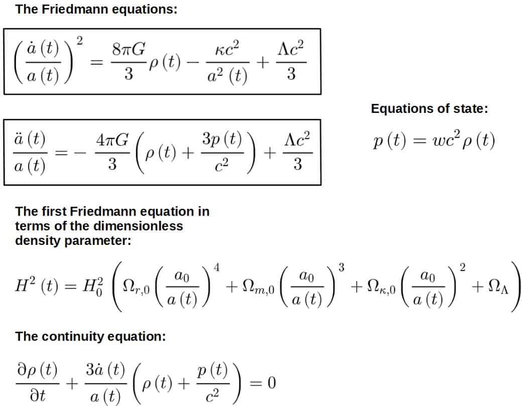
The most important equations we’ve discovered so far can be summarized as the following:
How To Solve The Friedmann Equations (Step-By-Step)
The Friedmann equations, at their heart, are differential equations we can use to solve for the scale factor a(t) – which then describes the expansion or time evolution of any particular universe on a large scale.
So, the goal of the Friedmann equations is to solve for the scale factor a(t).
However, the difficult part comes from the fact that we have three time-dependent variables in the Friedmann equations – the scale factor a(t), the energy density ρ(t) and the pressure p(t).
This is why we introduce an equation of state (as discussed earlier) – it allows us to eliminate one of the variables, namely, express pressure in terms of density.
By doing this, we’re then left with two equations – the two Friedmann equations – and two time-dependent variables, a(t) and ρ(t), which we can solve from the Friedmann equations.
Typically, we use the second Friedmann equation to solve for the density ρ(t) in terms of the scale factor a(t) and insert this into the first Friedmann equation to solve for a(t).
However, instead of the second Friedmann equation, we can equivalently use the continuity equation to find ρ(t) in terms of a(t). This is what we did earlier in this article.
So, to summarize, here are the rough steps for solving the Friedmann equations:
- Pick a particular universe model with scalar curvature parameter κ and some form(s) of energy.
- Write down an equation of state that relates pressure to energy density.
- Plug the pressure in terms of energy density into the second Friedmann equation or equivalently, into the continuity equation.
- Solve for the energy density in terms of the scale factor.
- Plug the energy density in terms of the scale factor into the first Friedmann equation. It is often easiest to use the first Friedmann equation expressed in terms of the dimensionless density parameters.
- Solve for the scale factor as a function of time.
Quick tip: If learning more about the math behind general relativity is of interest to you, I would highly recommend checking out my Mathematics of General Relativity: A Complete Course (link to the course page).
This course aims to give you all the mathematical tools you need to understand general relativity – and any of its applications. Inside the course, you’ll learn topics like tensor calculus in an intuitive, beginner-friendly and highly practical way that can be directly applied to understand general relativity.
Important Solutions of The Friedmann Equations
Perhaps the most important class of solutions to the Friedmann equations are those for a flat universe – a universe that corresponds to a scalar curvature parameter κ = 0.
This is because all current evidence suggests our own universe to be flat, which is why the flat universe solutions are the most widely considered in a lot of current research.
Below is a table showcasing solutions to the Friedmann equations in a flat universe for different types of energy.
| Matter-dominated | Radiation-dominated | Dark energy-dominated | |
| Equation of state | w=0 | w=\frac{1}{3} | w=-1 |
| Energy density | \rho\left(t\right)\propto a^{-3}\left(t\right) | \rho\left(t\right)\propto a^{-4}\left(t\right) | \rho\left(t\right)\propto a^0\left(t\right) |
| Scale factor | a\left(t\right)\propto t^{\frac{2}{3}} | a\left(t\right)\propto t^{\frac{1}{2}} | a\left(t\right)\propto e^t |
For open and closed universes, solutions to the Friedmann equations are slightly more complicated and require the use of so-called conformal time. You’ll find some discussion of open and closed universes later.
What Do The Friedmann Equations Predict?
In this section, we will consider how the Friedmann equations can be used to predict various things about our own universe, such as the eras of our universe’s history, the age of our universe and so on.
We’ll also consider the interesting question of how our universe might end as well (at least how the Friedmann equations would predict) as well as how different types of universes will end, depending on their curvature.
Let’s get started!
Eras of the Universe
Because the energy density of different forms of energy in the universe evolve differently through time, it is natural to ask what our own universe specifically is made of.
It actually turns out that our universe was dominated by a single component in different epochs of its history – the dominant form of energy in our universe was different at different times.
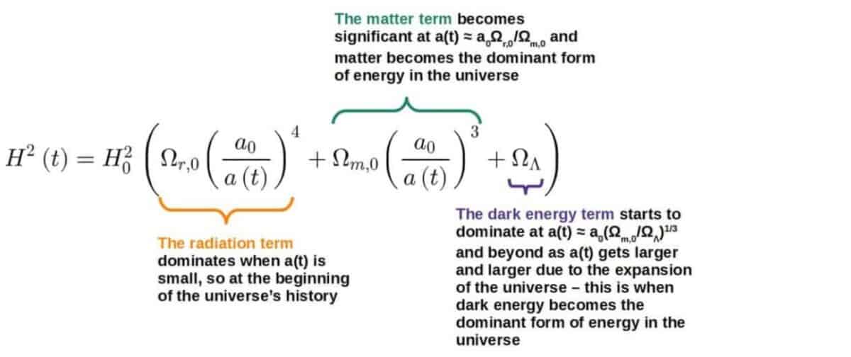
Considering only the contribution of “stuff” (so ignoring how the curvature affects things – after all, our own universe looks to be flat from what we observe), we can find periods of time when each of the three components singularly dominate.
- First we have the radiation-dominated era, for times such that 0 < a(t) < a0Ωr,0/Ωm,0.
- After, matter starts to become more important around the time when a(t) ≈ a0Ωr,0/Ωm,0.
- Matter has its time to shine and with the matter-dominated era existing for a0Ωr,0/Ωm,0 < a(t) < a0(Ωm,0/ΩΛ)1/3
- In the end, as a(t) gets larger and larger, all terms like 1/a2(t), 1/a3(t) and 1/a4(t) get smaller and smaller and we’re left only with the dark energy contribution: dark energy dominates for the times when a(t)>a0(Ωm,0/ΩΛ,0)1/3.
- Today, our universe is already in the “dark energy-dominant era” – the universe will keep on expanding due to dark energy being the dominant form of energy in our universe today.
Now, where do these “eras of the universe” come from?
Well, we can quite easily see this from the first Friedmann equation expressed in terms of the dimensionless density parameters (this is why this form of the Friedmann equation turns out to be extremely convenient):
Age of The Universe
Speaking of “today”, how old is our universe? Do the Friedmann equations give us an answer to this?
They do indeed! We can use experimental observations to aid us in this calculation.
First, within a very small margin of error, our universe appears to be flat so we can say that κ = ρκ = Ωκ = 0. One term in the Friedmann equations eliminated!
Now, here are some numbers for perspective: Ωr,0 ≈ 9×10⁻⁵, Ωm,0 ≈ 0.31, ΩΛ ≈ 0.69.
It also turns out that due to some symmetries of the FRW metric, we are free to set a0 = 1 (this just corresponds to picking a particular reference value for a0 and scaling the values of a(t) relative to this).
Using the eras of the universe from above, we can see that radiation dominated for times when a(t) < 9×10⁻⁵/0.31 = 2.9×10⁻⁴.
This will be for a very short amount of time so effectively, we can ignore the radiation contribution, leading us to the following form of the first Friedmann equation:
H^2\left(t\right)=\left(\frac{\dot{a}\left(t\right)}{a\left(t\right)}\right)^2=H_0^2\left(\frac{\Omega_{m{,}0}}{a^3\left(t\right)}+\Omega_{\Lambda}\right)With a bit of rearranging, we can mold this equation into the following form:
\frac{1}{\sqrt{a^2+\frac{\Omega_{m{,}0}}{\Omega_{\Lambda}}\frac{1}{a}}}\frac{da}{dt}=\sqrt{\Omega_{\Lambda}}H_0Reminder: \dot{a} is shorthand for da/dt.
We can now multiply by dt and integrate both sides.
Doing this, the left-hand side becomes an integral over a with integration limits going from 0 (the value of the scale factor effectively at the Big Bang) to 1 (the reference value of the scale factor we picked to be today).
The integration limits for the right-hand side will go from 0 to t0, the time that’s passed since the Big Bang (i.e. the current age of our universe). With these, we then get:
\int_{_0}^1\frac{1}{\sqrt{\frac{\Omega_{m{,}0}}{\Omega_{\Lambda}}\frac{1}{a}+a^2}}da=\sqrt{\Omega_{\Lambda}}H_0\int_{_0}^{t_0}dt=\sqrt{\Omega_{\Lambda}}H_0t_0The left-hand side can be calculated numerically to give a value of around 0.793513.
The last piece of the puzzle is Hubble’s constant – thanks to its relation to the velocities of galaxies in Hubble’s law, this can also be observationally measured!
The roughly agreed-upon value of Hubble’s constant is 68km/s/Mpc, where Mpc is a megaparsec (a peculiar unit used in astronomy) or in standard SI-units, about 2.2037×10⁻¹⁸.
This means that we can rearrange the above equation to solve for t0, the age of the universe. Doing this and plugging in the experimental values mentioned gives us the age of our universe:
t_0=\frac{1}{\sqrt{\Omega_{\Lambda}}H_0}\int_0^1\frac{1}{\sqrt{a^2+\frac{\Omega_{m{,}0}}{\Omega_{\Lambda}}\frac{1}{a}}}da\approx4.335\times10^{17}\ s=13.7\ \text{billion years}This, of course, is roughly the standard value of our universe’s age you may have seen before – the Friedmann equations gave us the correct answer!
On human scales, this age is above anything we could comprehend. But still, what if we were to go way beyond this into the future? What do the Friedmann equations predict then? Let’s consider this next!
End of the Universe
Is the universe eternal? Are we at risk of a Big Crunch? Will the universe expand forever, resulting in a Heat Death or Big Chill, as it is sometimes referred to?
All of this can be answered by the type of universe we live in.
Roughly, we can categorize universes into three categories, based on their spacial geometry:
- Open
- Flat
- Closed
If just for a moment, we rearrange the first Friedmann equation yet again (without absorbing the curvature term), we can mold it into:
\frac{H^2\left(t\right)}{H_0^2}=\frac{8\pi G\rho\left(t\right)}{3H_0^2}-\frac{c^2\kappa}{a^2\left(t\right)H_0^2}This equation is true at all times but in particular, it is true today (when the left-hand side will equal 1 since H(t)=H0).
If we evaluate this at t = t0, this equation simplifies greatly and we can use it to solve for the scalar curvature parameter κ:
1=\Omega-\frac{c^2\kappa}{a_0^2H_0^2}\ \ \Rightarrow\ \ \kappa=\frac{a_0^2H_0^2}{c^2}\left(\Omega-1\right)Here, we’ve used the definition of the dimensionless density parameter, Ω = 8πGρ(t)/3H02. Note that this parameter is for the total energy density of the universe, meaning it includes all forms of energy.
This means that depending on whether the dimensionless density parameter of the universe is less than, equal to, or greater than 1, the curvature is either negative, zero, or positive.
Geometrically, these situations are very different!
All positive curvature cases are similar and all negative curvature cases are roughly similar, so it’s enough for us to set κ=-1, 0, +1 to see the different possible outcomes.
These also go hand-in-hand with the three types of universe:
- Open universe has negative curvature (κ = -1)
- Flat universe has zero curvature (κ = 0)
- Closed universe has positive curvature (κ = 1)
Let’s look at how these different geometries affect how the universe evolves into the far future and how it might eventually end.
We’ll mostly be considering a matter-dominated universe, however, we’ll also discuss what happens to a flat universe dominated by dark energy later (which is what our own universe is observed to be).
Matter-Dominated Flat Universe, κ = 0
A flat universe with only matter has a rather elegant Friedmann equation (this comes from the first Friedmann equation written in terms of the density parameters, where the only non-zero density parameter is that of matter):
\left(\frac{\dot{a}\left(t\right)}{a\left(t\right)}\right)^2=\frac{H_0^2\Omega_{m{,}0}}{a^3\left(t\right)}We can take the square root and write the time-derivative fully to see we have something that looks just about solvable:
\frac{da\left(t\right)}{dt}=H_0\sqrt{\frac{\Omega_{m{,}0}}{a\left(t\right)}}This is what we call a separable ordinary differential equation in the ODE business – they are fortunately very solvable!
The solution turns out to be of the form:
a\left(t\right)\propto t^{\frac{2}{3}}Now, what does this mean? It simply means that as time passes, the scale factor in a flat universe just gets larger and larger: the universe expands forever!
We could do the same calculation with a universe full of radiation and we would find:
a\left(t\right)\propto t^{\frac{1}{2}}In reality, our universe is currently dominated by dark energy, which actually results in an exponential expansion rate instead of a polynomial one (this is explained more in the “Dark Energy” -section later).
However, the punchline here is that flat universes expand forever since their scale factors always increase with time.
As the universe expands, everything gets cooler and cooler with the entire universe eventually reaching thermodynamic equilibrium. We call this the Big Chill or the heat death of the universe.
We just so happen to be (most likely, based on astronomical observations) in a flat universe so the most probable ending for our own universe would be exactly this so-called Big Chill!
Matter-Dominated Closed Universe, κ = +1
The second type of universe we’ll consider is a closed universe. You may have heard of this type, or may even be able to guess why it is named so.
However, we’ll need to cover a few preliminaries before tackling this spacetime!
In order to make calculations easier, we will change coordinates to something called conformal time η (Greek letter “eta”).
Conformal time is a useful relativistic trick rather than being an observable quantity – it’s a mathematical “choice of coordinates” that allows us to do certain calculations.
We’ll define conformal time in terms of the scale factor as:
\eta=\int_0^t\frac{1}{a\left(t'\right)}dt'This may seem like an extremely random definition of an alternative time coordinate, but the usefulness of this comes from the fact that the time derivative of this conformal time quantity is given by (based on this definition):
\frac{d\eta}{dt}=\frac{1}{a\left(t\right)}This allows us to express many time derivatives in terms of the scale factor!
We will also, for convenience, use the convention c = 1 – that is, we set the speed of light equal to one.
This may seem bizarre at first but it is a commonly used convention as it simplifies many calculations and can always be added in again later by dimensional analysis.
Finally, since we’re considering a matter-dominated universe, we’ll have an energy density of the form ρm(t) = ρ0/a3(t).
Now, if we rearrange the first Friedmann equation for our closed universe, we find a slightly more complicated equation:
\left(\frac{\dot{a}\left(t\right)}{a\left(t\right)}\right)^2=\frac{8\pi G}{3}\frac{\rho_0}{a^3\left(t\right)}-\frac{1}{a^2\left(t\right)}You can try and separate this as best as you can to get:
\frac{da\left(t\right)}{dt}=\sqrt{\frac{8\pi G\rho_0}{a\left(t\right)}-1}To make progress, this is where we introduce conformal time – otherwise we wouldn’t be able to write down a closed form solution.
By the chain rule, we can express da(t)/dt as:
\frac{da\left(t\right)}{dt}=\frac{d\eta}{dt}\frac{da\left(\eta\right)}{d\eta}=\frac{1}{a\left(t\right)}\frac{da\left(\eta\right)}{d\eta}Plugging this into our Friedmann equation above, we find the following:
\frac{da\left(t\right)}{dt}=\sqrt{\frac{8\pi G\rho_0}{3a\left(t\right)}-1}\ \ \Rightarrow\ \ \frac{1}{\sqrt{\frac{8\pi G\rho_0}{3}a-a^2}}\frac{da}{d\eta}=1We can now integrate both sides:
\int_{ }^{ }\frac{1}{\sqrt{\frac{8\pi G\rho_0}{3}a-a^2}}da=\int_{ }^{ }d\eta=\etaThe left-hand side is difficult to work with but you can eventually find a closed form expression for the integral (the calculation isn’t very enlightening so I won’t go into detail here).
In the end, we find that:
\eta=\ \sin^{-1}\left(\frac{3a}{4\pi G\rho_0}-1\right)+\frac{\pi}{2}Now we just have to rearrange this and solve for the scale factor to see the fate of the closed universe!
Using the fact that sin(x-π/2)=-cos(x), we have:
a\left(\eta\right)=\frac{4\pi G\rho_0}{3}\left(1-\cos\eta\right)Note that at η=0 and η=2π, we have a(0) = a(2π) = 0. This is completely different to the flat universe!
The closed universe has a Big Bang, it expands and reaches a maximum scale factor of amax=4πGρ0/3 and then shrinks again, resulting in what is typically called a Big Crunch.
So, the lifetime of a closed universe is finite with everything eventually collapsing together into a singular point.
You may be wondering if this happens only because we chose a matter-dominated universe. If we instead considered a radiation-dominated closed universe, we would find:
a\left(\eta\right)\propto\sin\etaA radiation-dominated closed universe has exactly the same interpretation and fate as one filled with matter – a finitely lived universe.
Matter-Dominated Open Universe, κ = -1
The final category of universes for us to explore is the open universe.
The calculation here follows exactly the same procedure with the same tricks as for the closed universe.
The resulting integral equation is almost identical, except for a crucial sign change under the square root which changes the inevitable fate of the universe (this sign change comes from having κ = -1 instead of +1 like we did for the closed universe):
\int_{ }^{ }\frac{1}{\sqrt{\frac{8\pi G\rho_0}{3}a+a^2}}da=\int_{ }^{ }d\eta=\ \etaThe consequence of this sign flip is that the universe is saved from a crunching fate! We can see this by performing the above integral, which gives a very similar result:
a\left(\eta\right)=\frac{4\pi G\rho_0}{3}\left(\cosh\eta-1\right)However, the crucial difference here is that we have a hyperbolic cosine function (which is NOT periodic but increasing) instead of a cosine, which would be periodic.
For those of you who are familiar with hyperbolic and trigonometric functions, you may have guessed that a sign change would swap our result from a trigonometric to a hyperbolic one.
A radiation-dominated open universe follows the same pattern as the radiation-dominated closed universe, with a “sine” instead of a “cosine” (hyperbolic in this case):
a\left(\eta\right)\propto\sinh\etaBut what do these results mean for the fate of an open universe?
If we think on (conformal) timescales where η gets large (which corresponds to saying that the universe evolves into the far future), we can use the approximations:
\sinh\eta\approx\cosh\eta\approx\frac{1}{2}e^{\eta}This describes a scale factor that grows and grows with time – we’ve found another expanding universe!
So, an open universe will also expand forever, resulting in a Big Chill just like for a flat universe.
Dark Energy
Let’s consider one final contributor: dark energy.
The first Friedmann equation with an explicit cosmological constant term reads:
H^2\left(t\right)=\frac{8\pi G}{3}\rho\left(t\right)+\frac{\Lambda c^2}{3}If we have either a flat or open geometry, then we have a universe that will continue expanding forever as we have just seen before. But what causes this?
Well, we know that any non-cosmological constant form of energy density (matter, radiation, curvature) will be diluted by the expansion of spacetime.
This means that as time passes in the above equation, ρ(t) will start to get smaller and smaller (reminder; ρ(t) ∝ a-3(t) for radiation, ρ(t) ∝ a-3(t) for matter and ρ(t) ∝ a-2(t) for curvature).
If we’re considering only an open or flat universe, we’re safe to consider arbitrarily long timescales.
The effect of this is that the Hubble parameter gets smaller over time – eventually, the only meaningful contributor to the first Friedmann equation will be the cosmological constant term:
\left(\frac{\dot{a}\left(t\right)}{a\left(t\right)}\right)^2\approx\frac{\Lambda c^2}{3}At this point, the first Friedmann equation is completely solvable and we find the solution to be:
a\left(t\right)=a_0e^{\sqrt{\frac{\Lambda c^2}{3}}\left(t-t_0\right)}The interpretation of this is that as time passes, dark energy eventually becomes the dominant form of energy in a flat or open universe and along with this, the scale factor grows at an exponential rate.
So, the universe doesn’t just expand – the expansion rate itself increases exponentially with time. This again will result in a heat death for the universe, but much much faster than if dark energy wasn’t there.
In fact, at the current age of our universe (which is estimated to be flat), we’re at exactly this state – our own universe is expanding at an exponentially accelerating rate.
The key point with all of this is that if we have a non-zero cosmological constant (which describes dark energy), the universe will end up expanding forever at an exponential rate.
The claim I made at the beginning of this article about dark energy is now clearly laid out: dark energy drives the expansion of the universe!
Even as time passes and all other forms of energy density have been diluted to the point of negligibility, dark energy will continue to be produced by the ever expansion of the universe and that dark energy will power the universe’s expansion.
All of this we were able to predict from the Friedmann equations!
Cameron Bunney
I’m a third year PhD student at University of Nottingham, where I also studied my MMath. My main research focus is on curved spacetime QFT and the Unruh effect in analogue gravity systems. I have a soft spot for all kinds of math and physics, from number theory to mathematical biology and everything in between! Aside from research and recreational math, I enjoy playing piano and studying languages.
This article has been co-authored by Cameron Bunney.
